​

Preparation

This project aims on using Deep Learning with Kullback-Leibler Divergence. Some basic packages are required for this project. The aim of the following chunk is to install required packages such as lifelines, sklearn-pandas and torchtuples. Note that pycox is built based on torchtuples.

pwd
pip install lifelines
pip install sklearn-pandas
pip install torchtuples
pip install optunity
pip install statsmodels --upgrade
pip install pycox

We have used the API called google.colab.drive to get the software. Currently it is a series of python codes that wrapping necessary components for the experiments.

from google.colab import drive

drive.mount("/content/drive")

%cd "/content/drive/MyDrive/Kevin He"

data_simulation is the simulation codes that used for simulating data for our experiments, read_data is a class that can be used to generate different datasets, KLDL wraps necessary components.

import os
import sys
import time

import numpy as np
import pandas as pd
import matplotlib.pyplot as plt
import torch # For building the networks
import torch.nn as nn
import torch.nn.functional as F
import torchtuples as tt

# For preprocessing
from random import sample
# from pycox.models import PMF
# from pycox.models import DeepHitSingle

import KLDL
from KLDL import NewlyDefinedLoss
from KLDL import NewlyDefinedLoss2
import data_simulation
import read_data
import Structure

# MNIST is part of torchvision
from torchvision import datasets, transforms

​

Data Preprocessing

​

Introduction

Survival Data has its own special data structure that requires special models to analyze. Usually, for one patient (one data point/individual in the dataset), we can define the information as $\{\mathbf Z_i, t_i, \delta^*_i\}_{i = 1}^n$, with $\mathbf Z_i$ the derived features (the combinations of all raw/baseline features, for example, the second-order term/interaction term of baseline features), $t_i$ is the observed time, and $\delta_i = 1$ means the individual has event time, which is $t_i$. $\delta_i = 0$ means the individual is censored, then $t_i$ is the censored time.

Due to the existing of time and censoring, we usually focus on modeling the time-related features, such as survival probability or hazard values. We can also provide with a probability of one patient dying in a given period (such as 1-year survival score and so on), and this case is really suitable for discrete-time model in reality.

In this part we have defined several datasets that used in our experiments.

Simulation Data

We have designed a series of simulation data, all three of them have the same features $[x_1, x_2, x_3]$ and the model can be defined as

$\lambda(t |x) = \lambda_0(t) \exp(g(x, t))$

but with different model assumptions about $g(x, t)$, and there are three sets of data:

• Model consists of only linear term with no time effect (Simulation Data 1):

$g(x, t) = 0.22 x_1 + 0.44 x_2 + 0.88 x_3$

• Model consists of only linear and non-linear term with no time effect (Simulation Data 2):

$g(x, t) = 0.22 x_1 + 0.44 x_2 + 0.88 x_3 + \frac 23 (x_0^2 + x_2 ^2 + x_0 x_1 + 2x_1 x_2)$

• Model consists of linear, non-linear and time effect (Simulation Data 3):

$g(x, t) = 0.22 x_1 + 0.44 x_2 + 0.88 x_3 + \frac 23 (x_0^2 + x_2 ^2 + x_0 x_1 + 2x_1 x_2) + |0.2(x_0 + x_1) + 0.5 x_0 x_1|t$

Note that we also use simulation data 3 (with sample size $500, 5000, 30000$ for an experiment of hyperparameter tuning (to provide a suitable range of suggestions of tuning parameters), since this case is mostly close to the real case.

SUPPORT [data link]: The Study to Understand Prognoses Preferences Out comes and Risks of Treatment (SUPPORT) is a larger study that researches the survival time of seriously ill hospitalized adults. The support dataset is a random sample of 1000 patients from Phases I & II of SUPPORT (Study to Understand Prognoses Preferences Outcomes and Risks of Treatment). This dataset is very good for learning how to fit highly nonlinear predictor effects, imputing missing data, and for modeling 4 types of response variables:

• Binary (hospital death)

• Ordinal (severe functional disability)

• Continuous (total hospital costs or possibly study length of stay)

• Time until event (death) with waning effects of baseline physiologic variables over time. Patients are followed up to 5.56 years?

The dataset consists of 9,105 patients and 14 features for which almost all patients have observed entries (age, sex, race, number of comorbidi ties, presence of diabetes, presence of dementia, presence of cancer, mean arterial blood pressure, heart rate, respiration rate, temperature, white blood cell count, serum’s sodium, and serum’s creatinine), the bolded covariates are those recovered to have non-linear effects w.r.t. the risk score.

METABRIC [data link]:

Cancers are associated with genetic abnormalities. Gene expression measures the level of gene activity in a tissue and gives information about its complex activities. Comparing the genes expressed in normal and diseased tissue can bring better insights into the cancer prognosis and outcomes. Using machine learning techniques on genetic data has the potentials of giving the correct estimation of survival time and can prevent unnecessary surgical and treatment procedures.

The METABRIC dataset consists of gene expression data and clinical features for 1,980 patients, and 57.72 percent have an observed death due to breast cancer with a median survival time of 116 months [2]. We. prepare the dataset in line with the Immunohistochem- ical 4 plus Clinical (IHC4+C) test, which is a com- mon prognostic tool for evaluating treatment options for breast cancer patients [3]. We join the 4 gene indicators ( MKI67, EGFR, PGR, and ERBB2 ) with the a patient’s clin- ical features (hormone treatment indicator, radiotherapy indicator, chemotherapy indicator, ER-positive indicator, age at diagnosis)

For this dataset, we only follow the version from Deepsurv [4]

# Structure
	x1  x2  x3  ...  xp  durations  event
1
2
3
...

​

Read Data

read_data is the package that used for generating different kinds of data. It consists of simulation data and real data.

data_1 = read_data.simulation_data(option = "non linear non ph", n = 30000, grouping_number = 100)

data_1[50][1]

# Output

	x1	x2	x3	duration	event	temp
15000	-0.587828	0.798861	0.334242	5.022389	1	50
15001	-0.704029	0.565159	0.718257	1.860517	1	50
15002	-0.391265	-0.816136	-0.349752	20.338627	1	50
15003	-0.027009	0.389027	-0.283012	15.858289	0	50
15004	0.798371	-0.728038	0.828017	8.421642	1	50
...	...	...	...	...	...	...
15295	0.986675	0.563524	0.381906	0.996287	1	50
15296	0.647237	0.212581	0.775605	5.628805	1	50
15297	-0.186607	0.342446	-0.464537	30.000000	0	50
15298	0.765386	-0.855794	0.229596	10.114974	1	50
15299	-0.948526	-0.631569	0.142823	10.918161	0	50

support = read_data.support_data()
metabric = read_data.metabric_data()

For the further experiments, we design two schemes of prior data and local data to show the usage of our package. In general, prior data will have sufficient number of data points, but the model assumption/the number of features will be weaker, so here we generate prior data with only linear terms and proportional hazard assumption, but with 10000 data points. For local data, we generate 300 non linear and non proportional hazard data points, and we assume that this is the true model.

# Default grouping number is 0

data_local = read_data.simulation_data(option = "non linear non ph", n = 300)

prior_data = read_data.simulation_data(option = "linear ph", n = 10000)

​

Continuous to Discrete

Most experimental clinical data has continuous event time, which is not suitable for this project. Thus we apply the ways of discretization. More specifically, equi-distance or quantile-based.

time_intervals = 20

labtrans, prior_data = KLDL.cont_to_disc(prior_data, time_intervals = time_intervals)
data_local = KLDL.cont_to_disc(data_local, labtrans = labtrans, time_intervals = time_intervals)

prior_data

# Output

x1	x2	x3	duration	event
0	-0.686096	0.551481	-0.932677	14	0
1	-0.978083	-0.359753	0.053454	10	1
2	0.259453	0.763028	0.282278	7	1
3	-0.954624	0.390381	0.769304	10	1
4	0.502788	-0.473844	0.015149	13	1
...	...	...	...	...	...
9995	-0.804342	-0.374652	-0.291306	19	1
9996	-0.220712	-0.690892	-0.774906	4	1
9997	0.837798	-0.581770	0.629657	4	1
9998	0.633505	-0.266602	-0.436441	2	1
9999	-0.851903	-0.114422	0.078392	13	1
10000 rows × 5 columns

​

Model Training

​

Introduction: Methodology

Although the survival data structure is special, the model training procedure is still the same as traditional machine learning (we consider deep learning as one model of machine learning, since it focuses on approximating a function, but the goal of training this “function” is the same, which is trained a probability, a binary model in other words). Which requires

• Training, Validation and Test data.

• A loss function.

• The optimization algorithm, such as SGD, Adam, AdamW and RMSProp.

• Other tuning hyperparameters for the model.

Here we provide with a comprehensive introduction of our methodology. However you can skip this part if not interested.

​

Loss Function (Single Risk)

The loss function for discrete time model can be defined as

$l = \sum_{i = 1}^n \sum_{k = 1}^K Y_i(k)\left[ \log(1 - \lambda( \tau_k | \mathbf Z_i)) + \delta_i(k) \log \frac{\lambda (t_i | \mathbf Z_i)}{1 - \lambda (t_i | \mathbf Z_i)}\right]$

where $Y_i(k) = I(T_i \ge \tau_k), \delta_i(k) = I(T_i = \tau_k, \delta_i = 1)$. This is derived by knowing that

$L = \prod_{i = 1}^n L*_i = \prod_*{i = 1}^n f(t_i| \mathbf Z_i)^{\delta_i }S(t_i| \mathbf Z_i)^{1 - \delta_i}$

and $S(\tau_K|\mathbf Z_i) = \prod_{k = 1}^{K}[1 - \lambda(\tau_k|\mathbf Z_i)]$, $f(\tau_K|\mathbf Z_i) = \lambda(\tau_K|\mathbf Z_i)\prod_{k = 1}^{K - 1}[1 - \lambda(\tau_k|\mathbf Z_i)]$. This is also the loss function used by LogisticHazard (Nnet-Survival), and they choose to model hazard function by a neural network. As a comparison, Deephit models Probability Mass Function (PMF, $f$) instead.

For our model, we would like to use Kullback-Leibler (KL) Divergence as a way to incorporate model. In general, we can define it as

$D_{KL} (\psi_1, \psi_2) = \int \psi_1 \log \frac{\psi_1(x)}{\psi_2(x)} dx$

And it is defined as the information loss when $\psi_2$ is used to approximate $\psi^*_1$, a natural metric of measuring heterogeneity of two functions. So a lower value of $D_{KL} (\psi_1, \psi_2)$ means that the two functions have compatible information sources.

For our model, we will consider the two functions $\psi_1, \psi_2$ as two probabilistic distributions. We take hazard values as our interest and we will assume that we have two hazard functions $\boldsymbol \lambda, \tilde \lambda$. To be more clear, given the individual $i$ and the time point $\tau_k$, we can find that

$\lambda(\tau_k | \mathbf Z_i) = P(T_i = \tau_k | T_i \ge \tau_k, \mathbf Z_i)$

$1 - \lambda(\tau_k | \mathbf Z_i) = P(T_i > \tau_k | T_i \ge \tau_k, \mathbf Z_i)$

So conditional on $T_i \ge \tau_k$ and $\mathbf Z_i$, we can understand the hazard function as a binary variable, with probability of patient dying on time $\tau_k$ value $\lambda(\tau_k | \mathbf Z_i)$. The patient not dying on time $\tau_k$ value $1 - \lambda(\tau_k | \mathbf Z_i)$. Based on this observation, we can define our own KL divergence

$d_{k}\left( \boldsymbol {\tilde \lambda}, \boldsymbol \lambda ; \mathbf{Z}_{i}\right)=\tilde \lambda\left(\tau_k | \mathbf{Z}_{i}\right) \log \left\{\frac{\tilde \lambda\left(\tau_k | \mathbf{Z}_{i}\right)}{\lambda\left(\tau_k | \mathbf{Z}_{i}\right)}\right\}+\left\{1-\tilde \lambda\left(\tau_k | \mathbf{Z}_{i}\right)\right\} \log \left\{\frac{1-\tilde \lambda\left(\tau_k | \mathbf{Z}_{i}\right)}{1-\lambda\left(\tau_k | \mathbf{Z}_{i}\right)}\right\}$

with $\tilde \lambda$ the estimated hazard values from the external model (prior information) and $\lambda$ the hazard values from the internal model (and are unknown). It is time-dependent, which means varying the time point $\tau_k$ will lead to the different values of KL divergence since the hazard function depends on a given time point.

The cumulative hazard function for all dataset can be defined as

$D_{KL}(\boldsymbol {\tilde \lambda}, \boldsymbol \lambda) = \sum_{i = 1}^n \sum_{k = 1}^K Y_i(k) d_k(\boldsymbol {\tilde \lambda}, \boldsymbol \lambda; \mathbf x_i)$

and simple calculations lead to the result

$D_{K L}\left(\boldsymbol {\tilde \lambda}, \boldsymbol \lambda \right)=-\sum_{i=1}^{n} \sum_{k=1}^{K} Y_{i}\left(k \right)\left[\tilde{\lambda}\left(\tau_k | \mathbf Z_{i}\right) \log \left\{\frac{\lambda(\tau_k | \mathbf Z_i)}{1-\lambda(\tau_k | \mathbf Z_i)}\right\}+\log \left\{1-\lambda(\tau_k | \mathbf Z_i)\right\}\right] + C$

where $C$ is the constant, terms that not related to $\lambda(\tau_k|\mathbf Z_i), \forall, i, k$.

​

Loss Function (Competing Risk)

The way of modeling hazard value and using hazard value to define KL Divergence can also be smoothly transformed into our model. We will introduce only core changes of the loss function and leave more details to the paper as reference.

The contribution of the likelihood for an individual $i$ can be written as

$L_{i} = f_{r_i}(t_i)^{\delta_i} S(t_i)^{1- \delta_i} = \lambda_{r_{i}}\left(t_{i} | \mathbf{Z}_{i}\right)^{\delta_{i}}\left(1-\lambda\left(t_{i} | \mathbf{Z}_{i}\right)\right)^{1-\delta_{i}} \prod_{k=1}^{K-1}\left(1-\lambda\left(\tau_k | \mathbf{Z}_{i}\right)\right)$

where $t_i = \tau_K$ and $\lambda_{r_i}(t_i | \mathbf Z_i) = P(T^* = t_i, R = r_i \mid T^* \ge t_i, \mathbf Z_i)$, $\lambda(t_i|\mathbf Z_i) = \sum_{r = 1}^q \lambda_r(t_i|\mathbf Z_i) = P(T^* = t_i \mid T^* \ge t_i, \mathbf Z_i)$. $r_i$ is the index of causes that lead to the event.

The total loss function can be defined as

$l = \sum_{i = 1}^n \sum_{k = 1}^K Y_i(k)\left[ \log(1 - \lambda(\tau_k | \mathbf x_i)) + \sum_{r = 1}^q \delta_{i}^r(k) \log \frac{\lambda_{r} (t_i | \mathbf x_i)}{1 - \lambda (t_i | \mathbf x_i)}\right]$

where we define $\delta_i^r(k) = I(T_i = k, R_i = r, \Delta_i = 1)$.

Following the same way, but changing the binary distribution to multinomial (a clssification problem with $M + 1$ categories and the first $M$ elements have the probability $P(T = \tau_k, R = r | T \ge \tau_k, \mathbf Z_i), r = 1, 2, \ldots, M$, the last one is $P(T > \tau_k| T \ge \tau_k, \mathbf Z_i)$. We can define

$d_{k}\left( \boldsymbol {\tilde \lambda}, \boldsymbol \lambda ; \mathbf{Z}_{i}\right)= \sum_{r = 1}^M \tilde \lambda_r\left(\tau_k | \mathbf{Z}_{i}\right) \log \left\{\frac{\tilde \lambda_r\left(\tau_k | \mathbf{Z}_{i}\right)}{\lambda_r\left(\tau_k | \mathbf{Z}_{i}\right)}\right\}+\left\{1-\tilde \lambda\left(\tau_k | \mathbf{Z}_{i}\right)\right\} \log \left\{\frac{1-\tilde \lambda\left(\tau_k | \mathbf{Z}_{i}\right)}{1-\lambda\left(\tau_k | \mathbf{Z}_{i}\right)}\right\}$

and

$D_{KL}(\tilde{\boldsymbol{\lambda}}, \boldsymbol{\lambda}) = -\sum_{i=1}^{n} \sum_{k=1}^{K} Y_{i}(k)\left[\sum_{r = 1}^q \tilde \lambda_r \left(\tau_k \mid \mathbf{Z}_{i}\right) \log \left\{ \frac{\lambda_r(\tau_k | \mathbf Z_i)}{1 - \lambda(\tau_k|\mathbf Z_i)} \right\}+ \log \left\{1-\lambda\left(\tau_k | \mathbf{Z}_{i}\right)\right\} )\right]+C$

and

$l_\eta = \sum_{i = 1}^n \sum_{k = 1}^K Y_i(k)\left[ \log(1 - \lambda(k | \mathbf x_i)) + \sum_{r = 1}^q \frac{\delta_{i}^r(k) + \eta \tilde \lambda_r(k|\mathbf x_i)}{1 + \eta} \log \frac{\lambda_{r} (t_i | \mathbf x_i)}{1 - \lambda (t_i | \mathbf x_i)}\right]$

​

Optimizer

The optimizers can be different, but mainly we recommend Adam, AdamW and RMSProp. These three optimizers behave really similar in our test and we put all the three optimizers into the hyperparameter tuning.

​

Model Structure

The structure of neural network (The sizes of the parameters and the non-linear activation function in each layer) can be uniquely defined by a series of hyperparameters. We will provide with these options in the “hyperparameter tuning” section.

​

Proportional Version: 3 Link Functions

In Survival Analysis, there are 3 link functions that are frequently used for modeling. Although deep learning demonstrates a high flexibility of modeling non-linear, non-proportional data, in many cases where data is shown to have some statistical properties, using deep learning will instead lead to an inferior result. That is the reason we still provide with an option to simulate a function that can be proportional in some cases.

In general, we can uniformly define the model as

$h[d \Lambda (t, x)] = h[d \Lambda_0 (t)] + Z(t)' \beta$

where $h$ is a monotone-increasing and twice-differentiable function mapping $[0, 1]$ into $[-\infty, \infty]$ with $h(0) = - \infty$. Then we have the following 3 options:

1. $h(u) = \log (- \log (1 - u))$ (grouped relative risk model)
2. $h(u) = \log u$ (discrete relative risk model)
3. $h(u) = \log \frac u {1 - u}$ (discrete logistic model)

The code patch is shown below

if(option == "log-log"):
  input = input + torch.log(-torch.log(torch.sigmoid(self.a)))
  input = 1 - torch.exp(-torch.exp(input))
  return input
elif(option == "log"):
  input = input + torch.log(torch.sigmoid(self.a))
  input = torch.exp(input)
  return input
elif(option == "logit"):
  return torch.sigmoid(input + self.a)

Here is an illustration that shows the details of the last 3 layers:

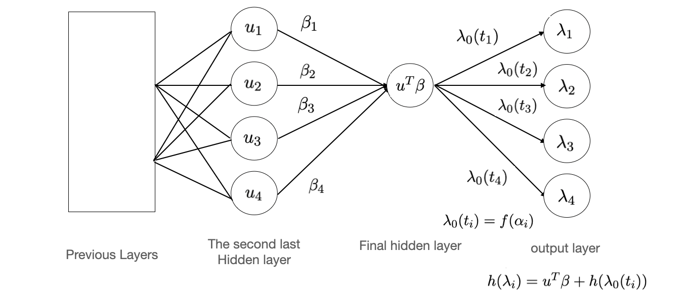
Here we assume that the number of nodes in the second last hidden layer is $4$, with $u_i, i = 1, 2, 3, 4$ the values that gotten by previous layers, $\beta_i$ is the weight connecting final hidden layer and the second last hidden layer, which is parameters that need to be estimated. Then a linear combination $u^T \beta$ is computed as the value of final hidden layer. After that, we define the weights connecting the last two layers as $f(\alpha_i)$, with $\alpha_i$ the parameters that originally initialized in the model, and $f$ be the pre-defined function that need to transform the weight to a baseline hazard value $\lambda_0(t_i)$ and it is determined by the link function we chosen. At last, the operation rules for the last two layers are defined by our own, following the formula. Note that if we assume the covariates for the input layer are time-independent, then since for each time point, the effect of covariates $u^T \beta$ is the same for each time point, we can guarantee that the neural network can simulate a proportional hazard model. However, if the covariates themselves are time-dependent, then no matter which design we use, the model will be non-proportional.

Non-proportional (Flexible): Why?

We can also provide with a flexible version (without carefully design of the structure for the last several layers except for a sigmoid function) of model structure

See the red and blue lines for weights connecting to $\lambda_1, \lambda_2$, where $\lambda_1$ means the hazard value at time point $\tau_1$, $\lambda_2$ means the hazard value at time point $\tau_2$. You can see although the $\lambda_1, \lambda_2$ will be connected with all the nodes in the last layer, the weights are totally different and they vary with time, so we can understand it as a model $y = x^\top \beta(t)$, with $\beta(t)$ different initial values when they are connected with values at different time points.

​

Link Function Comparisons

​

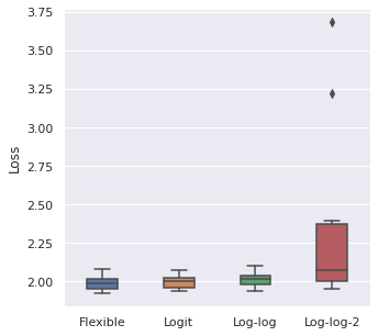
Prior Model

The core purpose of this project is to let user incorporate prior information by themselves. To incorporate the prior information, one should provide with a prior model with estimated parameters.

For example, suppose we have local features $[x_1, x_2, \ldots, x_{10}]$ but with prior model a partial model

$\hat y = x_1 + 2x_2 + 3x_3 + 2x_4 + 4x_5$

Then you should record the estimated parameters in the prior model and define the way for computing the prior information, whether it is an additive model ($x^T \beta$) or multiplictive model (for example, $\prod e^{x_i \beta_i}$). Which means you should store the parameter list as $[1, 2, 3, 2, 4, 0, 0, \ldots, 0]$, with coefficients of covariates not shown in the prior model $0$.

However, if you do not have a prior model, our software can also provide with a model with user-provided data, it can be all deep learning models that this software wraps, such as Deephit and LogisticHazard. We will show how to train a deep learning model in this tutorial, too.

optimizer`: optimizer, wrapped by `torchtuple

parameter_set = {
  hidden_nodes: 32,
  hidden_layers: 2,
  batch_norm: True,
  learning_rate: 0.0001,
  batch_size: 32,
}

model_prior = KLDL.prior_model_generation(
  prior_data,
  (parameter_set = parameter_set),
  (verbose = True)
)

# Output

0:	[1s / 1s],		train_loss: 7.2531,	val_loss: 6.8533
1:	[1s / 3s],		train_loss: 6.8347,	val_loss: 6.5090
2:	[1s / 4s],		train_loss: 6.4734,	val_loss: 6.1252
3:	[1s / 5s],		train_loss: 6.1032,	val_loss: 5.6914
4:	[1s / 6s],		train_loss: 5.6911,	val_loss: 5.3180
5:	[1s / 8s],		train_loss: 5.2043,	val_loss: 4.8396
6:	[1s / 9s],		train_loss: 4.7018,	val_loss: 4.1826

...

42:	[0s / 44s],		train_loss: 2.3292,	val_loss: 2.3421
43:	[0s / 45s],		train_loss: 2.3277,	val_loss: 2.3429

​

Hyperparameter Tuning: A Recommendation

It is recommended that we use hyperparameter tuning for the prior model (and also the local model). The parameters that can be used for tuning are listed below.

• number of hidden_nodes: This is the number of hidden nodes for each hidden layer, for saving the time of tuning we assume the hidden nodes for each layer are the same. In general tuning this parameter will have little obvious pattern of improvement given the same computational cost, so we only provide with three options $[32, 64, 128]$, which are also commonly used in other models used in Survival Analysis.

• number of hidden_layers: This is the number of hidden layers. Deeper neural network will have a better representation ability, which means easier to train a better model w.r.t. different metrics. However, it will also make the computational cost much higher. In general, we recommend user to have the number of layers to be chosen from $2$ to $5$, since if the neural network is too deep, it will make the training much more complicated and the gradient vanishing/exploding problem may be accumulating.

• whether use Batch Normalization or not: BatchNorm is recommended to deal with concept drift problem, it is strongly recommended when the trained network is deep (number of hidden_layers $\ge 2$).

• learning rate: The learning rate for the optimizer, it will vary a lot for different datasets. So our recommended values will also be multiple based on our test for different sizes of the dataset.

• batch size: Instead of computing the gradient using the whole dataset ($\frac 1n \sum_{i = 1}^n \nabla_\theta f(\mathbf x_i)$) or using only one data point (SGD, $\nabla_\theta f(\mathbf x_{i_k}))$, we compute the gradient for one batch of dataset ($\frac 1b \sum_{i \in I}\nabla_\theta f(\mathbf x_i), |I| = b$). The value of $b$ is chosen based on the size of data, but in general the maximum value of $b$ should not be over $0.05n$.

Here are some experiments showing the test results:

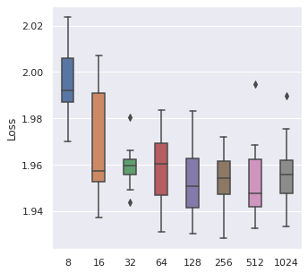
Batch Size

From left to right, top to bottom, we have generated 30000, 5000 and 500 data points following Simulation Data 3 and also a real dataset SUPPORT. We have found that about $5\%$ of the size is a maximum boundary for the mini-batch training, for the minimum, it is a little hard to determine, but $0.1 - 1\%$ of the size is a safe range, which means that if you have a data size of 10000, then we recommend tuning the batch size from 10 to 500.

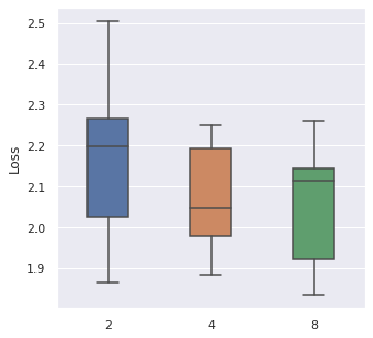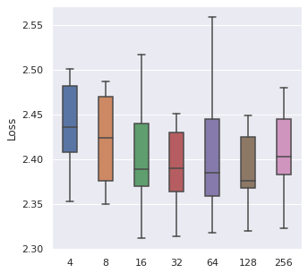The time cost can also be viewed in the same order, too. A take-home message is that: approximately $1\%$ of the data size can be set as the batch size when we also consider the time cost.

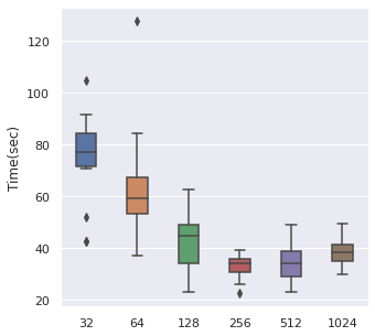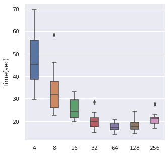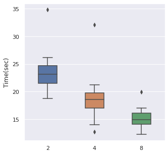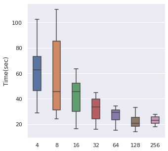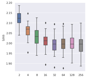
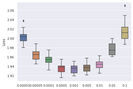
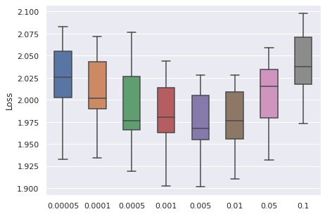
Learning Rate

We have taken a series of values for potential learning rate, which are $[0.00001, 0.00005, 0.0001, 0.0005, 0.001, 0.005, 0.01, 0.05, 0.1]$, we have observed that the values from $0.0001$ to $0.05$ can be a proper range, so this will be our range for tuning.

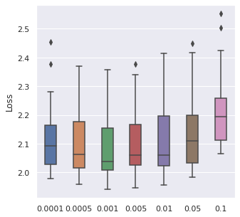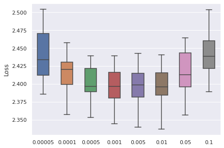The time cost can be viewed with the same order. In general, higher learning rate means faster convergence, so people can tune from the largest to the smallest learning rate for saving time.

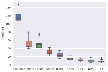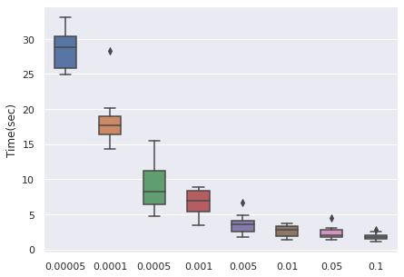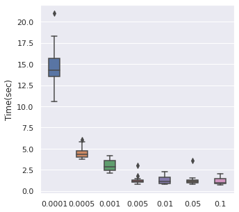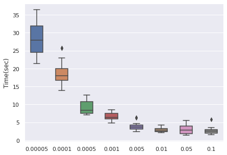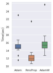
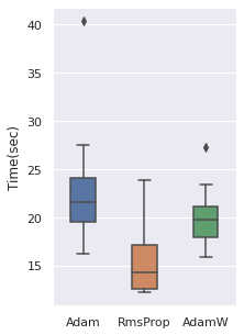
Optimizer

We have tried 4 optimizers (SGD, Adam, RMSProp, AdamW) and 3 are comparable, the other one is inferior. So these three optimizers will be used.

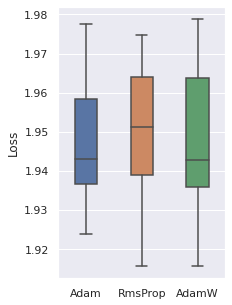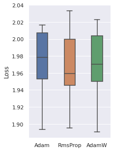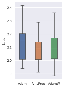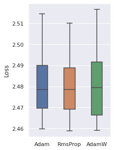The time cost can be viewed with the same order, note that RmsProp is the option with the least time cost.

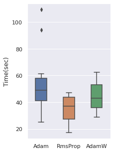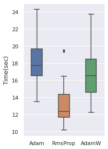Dropout Rate

We take $[0, 0.1, 0.25, 0.5]$ as potential values for tuning and for the first three values, there are no significant difference but they all behave better than the $0.5$ case. This is reason that for default hyperparameter tuning recommendation, we will use $[0, 0.1, 0.25]$ as 3 potential options.

The time cost can be viewed with the same order. No clear result is shown.

KLDL.hyperparameter_set_list(
  (hidden_nodes = [32, 64]),
  (hidden_layers = [2]),
  (batch_norm = [True]),
  (learning_rate = [0.001, 0.01]),
  (batch_size = [32])
)

# Output

[{'batch_norm': True,
  'batch_size': 32,
  'hidden_layers': 2,
  'hidden_nodes': 32,
  'learning_rate': 0.001},
 {'batch_norm': True,
  'batch_size': 32,
  'hidden_layers': 2,
  'hidden_nodes': 32,
  'learning_rate': 0.01},
 {'batch_norm': True,
  'batch_size': 32,
  'hidden_layers': 2,
  'hidden_nodes': 64,
  'learning_rate': 0.001},
 {'batch_norm': True,
  'batch_size': 32,
  'hidden_layers': 2,
  'hidden_nodes': 64,
  'learning_rate': 0.01}]

Below is a sketch of doing hyperparameter tuning. Due to the time limit, we do not test it in this tutorial.

# DO NOT RUN!!

best_model = None
best_score = 10000

set_list = KLDL.hyperparameter_set_list()
for i in set_list:
  log, model = KLDL.model_generation(data, parameter_set = i)
  score = log.to_pandas().val_loss.min()
  if(score < best_score):
    best_score = score
    best_model = model

​

Cross Validation (CV)

After we train a prior model, we need to decide the value of $\eta$ to see how much we can ‘trust’ the information from the prior model. Mathematically, $l_\eta = \frac{l - \eta l_{KL}}{\eta + 1}$, so we can understand the combined loss as ‘1 local information and $\eta$ prior information’. For better understanding, if $\eta = 1$, this means the weights for local and prior information are 50-50 ($\frac 1 {1 + 1} = \frac 12 = 50\%$). The CV will be done 5-fold and the metrics will be averaged. Currently C-index is used, measured on a separate dataset in the local data.

eta_list = [0.1, 1, 5]
eta, df_train, df_test, (x_test = KLDL.cross_validation_eta(data_local, eta_list, model_prior))

​

Local Model Training

We will train two versions of model (same model structure, only difference is whether we have prior information). As a reminder, we firstly have the prior model to get the prior information, which is the time-dependent hazard function at each time point for each individual obtained by external model, and then we compute the loss function with the aid of prior information and selected $\eta$.

We will use the selected $\eta$ and the trained prior model to train our local model. Note that we will not use the same splitting as what have shown before (The df_train and df_test that output from KLDL.cross_validation_eta.

parameter_set = {
  hidden_nodes: 32,
  hidden_layers: 2,
  batch_norm: True,
  learning_rate: 0.005,
  batch_size: 32,
}

df_train = data_local.copy()

df_val = df_train.sample((frac = 0.2))
df_train = df_train.drop(df_val.index)

mapper = KLDL.mapper_generation((cols_standardize = ['x1', 'x2', 'x3']))

x_train = mapper.fit_transform(df_train).astype('float32')
x_val = mapper.transform(df_val).astype('float32')

y_train = (x_train, df_train['duration'].values, df_train['event'].values)
y_val = (x_val, df_val['duration'].values, df_val['event'].values)

model = KLDL.model_generation(
  x_train,
  x_val,
  y_train,
  y_val,
  (eta = eta),
  (model_prior = model_prior),
  (parameter_set = parameter_set),
  (verbose = True)
)

We can also train a normal model, which is the model that will not incorporate prior information.

# The data structure of y_train and y_val is different

get_target = lambda df: (df['duration'].values, np.array(df['event'].values, dtype = np.float32))

y_train = get_target(df_train)
y_val = get_target(df_val)

# Flexible v.s. Proportional: Option
model_2 = KLDL.model_generation(x_train, x_val, y_train, y_val, with_prior = False, parameter_set = parameter_set, verbose = True, option = "logit")

# Output

0:	[0s / 0s],		train_loss: 7.7840,	val_loss: 6.9216
1:	[0s / 0s],		train_loss: 5.5561,	val_loss: 5.1591
2:	[0s / 0s],		train_loss: 4.7117,	val_loss: 4.5906
3:	[0s / 0s],		train_loss: 4.0036,	val_loss: 4.0526
4:	[0s / 0s],		train_loss: 3.5878,	val_loss: 3.4386
5:	[0s / 0s],		train_loss: 3.0214,	val_loss: 3.0906
6:	[0s / 0s],		train_loss: 2.8459,	val_loss: 2.8541

...

69:	[0s / 2s],		train_loss: 1.9728,	val_loss: 2.2558
70:	[0s / 2s],		train_loss: 1.9611,	val_loss: 2.2500

​

Evaluation

​

Introduction: Methodology

In Survival Analysis, there are so many possible metrics that can be used for evaluation. We hereby introduce them and same, for readers who are not interested, you can skip this part.

​

Harrell’s C-index

The core principle for Harrell’s C-index is given a set of comparable pairs, the individual with longer event time should have a smaller survival probability. To be more concrete, it is defined as

$C = P(S(t|\mathbf Z_i(\mathbf t)) < S(t|\mathbf Z_j(\mathbf t)) \mid T_i < T_j \land \Delta_i = 1) = \frac{\pi_{conc}}{\pi_{comp}}$

where $\pi_{comp} = P(T_i < T_j \land \Delta_i = 1)$ and $\pi_{conc} = P(S(t|\mathbf x_i(\mathbf t)) < S(t|\mathbf x_j(\mathbf t)) \land T_i < T_j \land \Delta_i = 1)$. This comes from the concept of area under curve (AUC).

For computation, we define

$\operatorname{comp}_{i j}=I\left\{t_{i}<t_{j} \& d_{i}=1\right\}+I\left\{t_{i}=t_{j} \& d_{i}=1 \& d_{j}=0\right\}$

and

$\text {conc}_{ij}=I\left\{z\left(\mathbf{x}_{i}\right)>z\left(\mathbf{x}_{j}\right)\right\} \cdot \operatorname{comp}_{ij}$

we can have the computation steps

$c=\frac{\sum_{i=1}^{n-1} \sum_{j=i+1}^{n}\left(\operatorname{conc}_{i j}+\operatorname{conc}_{j i}\right)}{\sum_{i=1}^{n-1} \sum_{j=i+1}^{n}\left(\operatorname{comp}_{i j}+\operatorname{comp}_{j i}\right)}=\frac{\sum_{i=1}^{n} \sum_{j=1 ; j \neq i}^{n} \operatorname{conc}_{i j}}{\sum_{i=1}^{n} \sum_{j=1 ; j \neq i}^{n} \operatorname{comp}_{i j}}$

​

Antolini’s C-index

Antolini’s C-index is one commonly used time-dependent C-index, note that for Harrell’s version, it only provides with a measurement of C-index at a given time.

Note that

$\operatorname{AUC}\left(t_{(k)}\right)=\operatorname{Pr}\left\{S\left(t_{(k)} \mid \mathbf{Z}_{i}(\mathbf{t})\right)<S\left(t_{(k)} \mid \mathbf{Z}_{j}(\mathbf{t})\right) \mid D_{i}\left(t_{(k)}\right)=1 \& D_{j}\left(t_{(k)}\right)=0\right\}$

is defined as the discrimination ability of $S(t_{(k)}, \mathbf Z(t))$. Then we define the time-dependent C-index as

$C^{\mathrm{td}}=\frac{\sum_{k=0}^{K} \operatorname{AUC}\left(t_{(k)}\right) \cdot w\left(t_{(k)}\right)}{\sum_{k=0}^{K} w\left(t_{(k)}\right)}$

where

$w\left(t_{(k)}\right)=\operatorname{Pr}\left\{D_{i}\left(t_{(k)}\right)=1 \& D_{j}\left(t_{(k)}\right)=0\right\}$

Proofs show that

$C^{\mathrm{td}}=\frac{\pi_{\mathrm{conc}}^{\mathrm{td}}}{\pi_{\mathrm{comp}}}=\operatorname{Pr}\left\{S\left(T_{i} \mid \mathbf{X}_{i}(\mathbf{t})\right)<S\left(T_{i} \mid \mathbf{X}_{j}(\mathbf{t})\right) \mid T_{i}<T_{j} \& D_{i}=1\right\}$

where

$\pi_{\mathrm{comp}} = \sum_{k=0}^{K} w\left(t_{(k)}\right)$

and

$\pi_{\mathrm{conc}}^{\mathrm{td}}=\sum_{k=0}^{K} \operatorname{AUC}\left(t_{(k)}\right) \cdot w\left(t_{(k)}\right)$

For computation, the term $\operatorname{comp}_{ij}$ is defined the same as Harrell’s C-index. Define also

$\operatorname{conc}_{i j}^{\mathrm{td}}=I\left\{S\left(t_{i} \mid \mathbf{x}_{i}(\mathbf{t})\right)<S\left(t_{j} \mid \mathbf{x}_{j}(\mathbf{t})\right)\right\} \cdot \operatorname{comp}_{i j}$

Then we can compute this value as

$c^{\mathrm{td}}=\frac{\sum_{i=1}^{n} \sum_{j=1 ; j \neq i}^{n} \operatorname{conc}_{i j}^{\mathrm{td}}}{\sum_{i=1}^{n} \sum_{j=1 ; j \neq i}^{n} \operatorname{comp}_{i j}}$

​

Uno’s C-index

​

Integrated Brier Score (IBS)

IBS is also a metric that measures the difference between true and predicted survival value and the idea comes from MSE.

Generally, we have

$\operatorname{BS}(t^*) = \frac 1n \sum_{i = 1}^n (I(T_i > t^*) - \hat \pi(t^* | \mathbf x_i))^2$

For censoring case, there are altogether 3 cases

• $T_i \le t^* \land \delta_i = 1 \Rightarrow [0 - \hat \pi(t^* | \mathbf x_i)]^2$

• $T_i > t^* \land \delta_i = 0 / 1 \Rightarrow [1 - \hat \pi(t^* | \mathbf x_i)]^2$

• $T_i \le t^* \land \delta_i = 0 \Rightarrow No Solution$

To remedy the 3-rd case, the inverse weights are added, which means the Brier Score under censoring (assuming random censorship) is defined as

$\operatorname{BS^c}(t^*) = \frac 1n \sum_{i = 1}^n \{(0 - \hat \pi(t^*|\mathbf x_i))^2 I(T_i \le t^*, \delta_i = 1)(1 / \hat G(T_i)) + (1 - \hat \pi(t^*|\mathbf x_i))^2I(T_i > t^*)(1 / \hat G(t^*))\}$

where $\hat G(t)$ denotes the KM estimate of the censoring distribution.

The integrated version is defined as

$\operatorname{IBS} = \frac 1 {t_{max} - t_{min}}\int_{t_{min}}^{t_{max}} BS^c(t)dt$

​

Integrated Negative Binomial log-likelihood (INBLL)

Similar for IBS, we have

$\operatorname{BLL}(t^*) = \frac 1n \sum_{i = 1}^n \{\log(1 - \hat \pi(t^* | \mathbf x_i)) I(T_i \le t^*, \delta_i = 1)(1 / \hat G(T_i)) + \log(\hat \pi(t^* | \mathbf x_i))I(T_i > t^*)(1 / \hat G(t^*))\}$

And

$\operatorname{INBLL} = -\frac 1 {t_{max} - t_{min}}\int_{t_{min}}^{t_{max}} BLL(t)dt$

​

Usage of Software

durations_test, (events_test = get_target(df_test))

concordance_td_local,
  integrated_brier_score_local,
  (integrated_nbll_local = KLDL.evaluation_metrics(
    x_test,
    durations_test,
    events_test,
    model_local
  ))
concordance_td_prior,
  integrated_brier_score_prior,
  (integrated_nbll_prior = KLDL.evaluation_metrics(
    x_test,
    durations_test,
    events_test,
    model_prior
  ))
concordance_td,
  integrated_brier_score,
  (integrated_nbll = KLDL.evaluation_metrics(x_test, durations_test, events_test, model))

print('The C-index for local without prior: ', concordance_td_local)
print('The C-index for local with prior: ', concordance_td)
print('The C-index for prior: ', concordance_td_prior)
print('The IBS for local without prior: ', integrated_brier_score_local)
print('The IBS for local with prior: ', integrated_brier_score)
print('The IBS for prior: ', integrated_brier_score_prior)
print('The INBLL for local without prior: ', integrated_nbll_local)
print('The INBLL for local with prior: ', integrated_nbll)
print('The INBLL for prior: ', integrated_nbll_prior)

# Output

The C-index for local without prior:  0.6533665835411472
The C-index for local with prior:  0.71238570241064
The C-index for prior:  0.7115544472152951
The IBS for local without prior:  0.142921780409424
The IBS for local with prior:  0.1502653697125696
The IBS for prior:  0.14910643935465429
The INBLL for local without prior:  0.43334645529434623
The INBLL for local with prior:  0.4544365897650282
The INBLL for prior:  0.451068920566815

​

Future Work

1. Interpolation: From discrete survival probability to continuous for fair comparison.

2. Different link functions: Modify the link functions to adapt to different kinds of data (which data adapts to which link functions).

3. Options for avoiding data expansion (required interface of C++ and Python).

4. Hyperparameter Tuning based on Random Search.

​

Reference

1. Knaus WA, Harrell FE, Lynn J et al. (1995): The SUPPORT prognostic model: Objective estimates of survival for seriously ill hospitalized adults. Annals of Internal Medicine 122:191-203.

2. urtis C, Shah SP, Chin S-F, Turashvili G, Rueda OM, Dunning MJ, Speed D, Lynch AG, Samarajiwa S, Yuan Y, et al. The genomic and transcriptomic architecture of 2,000 breast tumours reveals novel subgroups. Nature. 2012;486(7403):346–52.

3. akhanpal R, Sestak I, Shadbolt B, Bennett GM, Brown M, Phillips T, Zhang Y, Bullman A, Rezo A. Ihc4 score plus clinical treatment score predicts locoregional recurrence in early breast cancer. The Breast. 2016;29:147–52.

4. Katzman, J.L., Shaham, U., Cloninger, A., Bates, J., Jiang, T. and Kluger, Y., 2018. DeepSurv: personalized treatment recommender system using a Cox proportional hazards deep neural network. BMC medical research methodology, 18(1), pp.1-12.

5. Ioffe, Sergey, and Christian Szegedy. “Batch normalization: Accelerating deep network training by reducing internal covariate shift.” International conference on machine learning. PMLR, 2015.

6. Kvamme, Håvard, and Ørnulf Borgan. “Continuous and discrete-time survival prediction with neural networks.” arXiv preprint arXiv:1910.06724 (2019).

7. Gensheimer, Michael F., and Balasubramanian Narasimhan. “A scalable discrete-time survival model for neural networks.” PeerJ 7 (2019): e6257.

8. Wang, Di, Wen Ye, and Kevin He. “Kullback-Leibler-Based Discrete Relative Risk Models for Integration of Published Prediction Models with New Dataset.” Survival Prediction-Algorithms, Challenges and Applications. PMLR, 2021.

9. Antolini, Laura, Patrizia Boracchi, and Elia Biganzoli. “A time‐dependent discrimination index for survival data.” Statistics in medicine 24.24 (2005): 3927-3944.

10. Uno, Hajime, et al. “On the C‐statistics for evaluating overall adequacy of risk prediction procedures with censored survival data.” Statistics in medicine 30.10 (2011): 1105-1117.

11. Graf, Erika, et al. “Assessment and comparison of prognostic classification schemes for survival data.” Statistics in medicine 18.17‐18 (1999): 2529-2545.

12. Bergstra, James, and Yoshua Bengio. “Random search for hyper-parameter optimization.” Journal of machine learning research 13.2 (2012).

13. Tutz, Gerhard, and Matthias Schmid. Modeling discrete time-to-event data. New York: Springer, 2016.

14. Kalbfleisch, John D., and Ross L. Prentice. The statistical analysis of failure time data. John Wiley & Sons, 2011.

15. Lee, Changhee, et al. “Deephit: A deep learning approach to survival analysis with competing risks.” Proceedings of the AAAI conference on artificial intelligence. Vol. 32. No. 1. 2018.