​

Abstract

Profiling of healthcare providers (such as dialysis facilities or physicians) is of nationwide importance. This analysis may lead to changes in budgeting allocations and even suspension. Existing profiling approaches assume the between-provider variation is entirely due to the quality of care (e.g. the risk adjustment is perfect), which is often invalid. As a result, these methods disproportionately identify larger providers, although they need not be “extreme.” To fairly assess healthcare providers, appropriate statistical methods are in urgent need to account for the unexplained variation due to imperfect risk adjustment. In response, we develop a novel individualized empirical null approach for profiling healthcare providersc to account for the unexplained between-provider variation due to the imperfect risk adjustment, which is robust to outlying providers. The proposed individualized empirical null approach is adaptable to different provider sizes, as the total variation used for assessing provider effects usually changes with the provider’s own sample size.

​

1 Introduction

Large-scale electronic health records derived from national disease registries have proven useful for measuring health care processes and outcomes. In order to monitor and quantify such differences, many patient level clinical outcomes are being closely monitored and summarized into provider-level measures, for example, in the Dialysis Facility Compare Program by Centers for Medicare & Medicaid Services (CMS). Provider profiling based on these clinical outcomes can help patients make more informed decisions as to their choice of providers, and also aid overseers and payers in identifying providers whose outcomes are worse or better than a normative standard, in order to signal the need for further reviews or to target quality improvement programs. The statistical analysis along with further reviews may lead to changes in budgeting allocations and even suspension for those providers with extremely poor outcomes. Thus, accurate profiling of healthcare providers with extreme performance is of nationwide importance (XX). Given the high stakes of such evaluations, it is crucial that the statistical methods for provider profiling appropriately account for differences in patient characteristics and suitably allow for unexplained variation due to imperfect risk-adjustment.

Our endeavor is motivated by the study of end-stage renal disease (ESRD). End-stage renal disease (ESRD) is one of the most deadly and costly diseases. In 2016 there were 726,331 prevalent cases of ESRD in the United States (?), which represents an increase of 80$\%$ since 2000. Between 2015 and 2016, Medicare fee-for-service (FFS) spending for beneficiaries with ESRD rose by 4.6$\%$ (Figure 1b), from $33.8$ billion to $35.4$ billion, accounting for 7.2$\%$ of overall Medicare paid claims. These high health care expenditures represent a major health care burden and are worthy of special scrutiny. In order to identify extreme (poor or excellent) performance and to intervene as necessary, outcomes of patients associated with dialysis facilities or physicians are routinely monitored most often by both government and private payers. This monitoring can help patients make more informed decisions, and can also aid consumers, stakeholders, and payers in identifying facilities where improvement may be needed, and even closing or ending those with extremely poor outcomes. For such purposes, both fixed effects (FE) and random effects (RE) approaches have been widely used. However, existing FE and RE approaches assume the between-provider variation is entirely due to the quality of care, which is often invalid; e.g. unobserved socioeconomic factors and comorbidities may differ substantially across providers and contribute to the between-provider variation. As a result, the usual standard normal distribution assumption for the null distribution of the test statistics is invalid, leading to large differences in subsequent profiling. In particular, the FE method disproportionately profiles larger providers, although their difference from the national average may not be clinically meaningful and such providers need not be “extreme.”

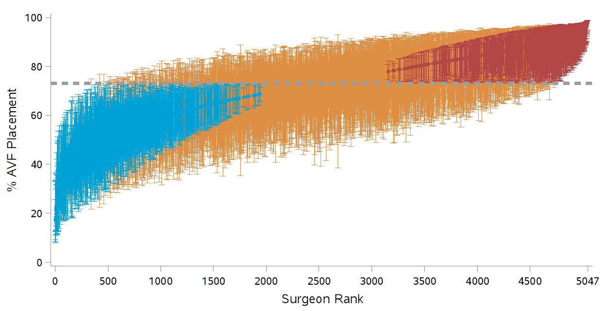
Figure 1: RE-based adjusted percentages and 95$\%$ confidence intervals; Dashed line: median value; Blue: significantly below; Red: significantly above.

---

The idea of empirical null was introduced in Efron (2004) in the context of multiple testing with a uniform null distribution. Kalbfleisch and Wolfe (2013) propose using the empirical null distribution of the FE-based Z-scores to assess outlying providers. Specifically, a robust estimation technique is applied to obtain the mean and variance estimates of the FE-based Z-scores, which can then be used as reference in hypothesis testing. However, in application with provider profiling, the total variation for assessing provider effects and the distribution of the test statistics usually change with the provider’s sample size. This leads to individualized null distributions for the test-statistics, precluding the application of existing empirical null approaches. To fairly assess providers, we propose an individualized empirical null approach, which is adaptable to different provider sizes and are robust to outlying providers. Linear models 3 are presented first to introduce the proposed framework, and our proposed method accommodates many other types of outcomes, such as hospital admissions and ED visits in a Poisson model and readmission in a logistic model. Our contribution to the literature can be summarized as follows: First, in recognition of the fact that risk-adjustment is never perfect, the proposed individualized empirical null approach accounts for the unexplained variation between providers. Second, the method is adaptable to different provider sizes and avoids the bias against large providers. Finally, the method incorporates the contamination of outliers, and is robust for identifying outlying providers.

​

2 Individualized Empirical Null for Linear Models

Let $Y_{ij}^*$ represent a continuous outcome for subject $j$ in provider $i$, $j = 1, \ldots, n_i$, where $n_i$ is the sample size for provider $i$. Consider an underlying linear regression model

where $\gamma_i$ is the provider effect, $\epsilon_{ij} {\sim} N (0, \sigma_w^2)$ is the random noise, $\textbf{X}_{ij}$ is a vector of patient characteristics, and the regression coefficient, $\boldsymbol\beta$, measure the within-provider relationship between the covariates and the response. Here $\alpha_i {\sim} N(0, \sigma_{\alpha}^2)$ is a random effect, which can be thought of as an unobserved confounders.

We note that, in profiling applications with national disease registries, the number of patients is large so that $\mu$, $\boldsymbol\beta$ and $\sigma_w$ can be precisely estimated. To simplify the notation, we proceed below as though their values are known. Let $Y_{ij}=Y_{ij}^*- \textbf{X}_{ij}^T\boldsymbol\beta$ be the risk adjusted response, so that the model becomes

​

2.1 FE and RE Approaches

The FE-based Z-score for a sharp null hypothesis $\alpha_i=0$ is $Z_{FE, i} = (\bar{Y}_i-\mu)/ ({\sigma}_w/\sqrt{n_i})$, where $\bar{Y}_i =\sum_{j=1}^{n_i}Y_{ij}/n_i$. Assuming that large values of $Y_{ij}$ correspond to poor outcomes, the $i$th provider is flagged as worse than expected if $Z_{FE, i}>z_{p}$, where $z_p$ is the upper $p$th quantile of the standard normal distribution. However, in practice, the empirical distribution of z-scores is more dispersed than the standard normal distribution (Figure 1a), a phenomenon known as over-dispersion. As illustrated in Figures 1b-1d, the variation of Z-scores is larger for providers with larger size. In fact, when the randomness of provider effects is taken into account, the marginal variance of the Z-scores is $1+n_i \sigma_{\alpha}^2/\sigma_w^2$, which is a linear function of the sample size $n_i$. The issue is that the FE approach assumes that the risk-adjustment is perfect, which, however, is often violated in practice. As a results, the usual standard normal distribution assumption for the null distribution is invalid, leading to large differences in subsequent profiling. In particular, the FE method disproportionately profiles larger providers, although their difference from the national average may not be clinically meaningful and such providers need not be “extreme.”

Alternatively, the RE approach is based on the best linear unbiased predictor (BLUP) arising from the “posterior” distribution of $\alpha_i$ given the data. The corresponding Z-score is given by $Z_{RE,i} = \sqrt{{R}_i} Z_{FE, i}$, where $R_i=\sigma_{\alpha}^2/({\sigma_{\alpha}^2+\sigma_w^2/n_i})$ plays the role of a shrinkage factor. The RE approach gives estimates with a smaller mean squared error than the FE estimate, which, however, is achieved at the cost of bias. The bias is especially substantial for providers with small sizes. Moreover, the RE-based Z-score suffers from the same problem as the FE approach and disproportionately profiles large providers. As illustrated in Figure 2, if a provider treats a sufficiently large number of patients, even a slight departure from the national norm is likely to be profiled as extreme. It should also be noted that the naive use of RE can lead to biased estimation of provider effects and regression coefficients when covariates are correlated with the provider effects.

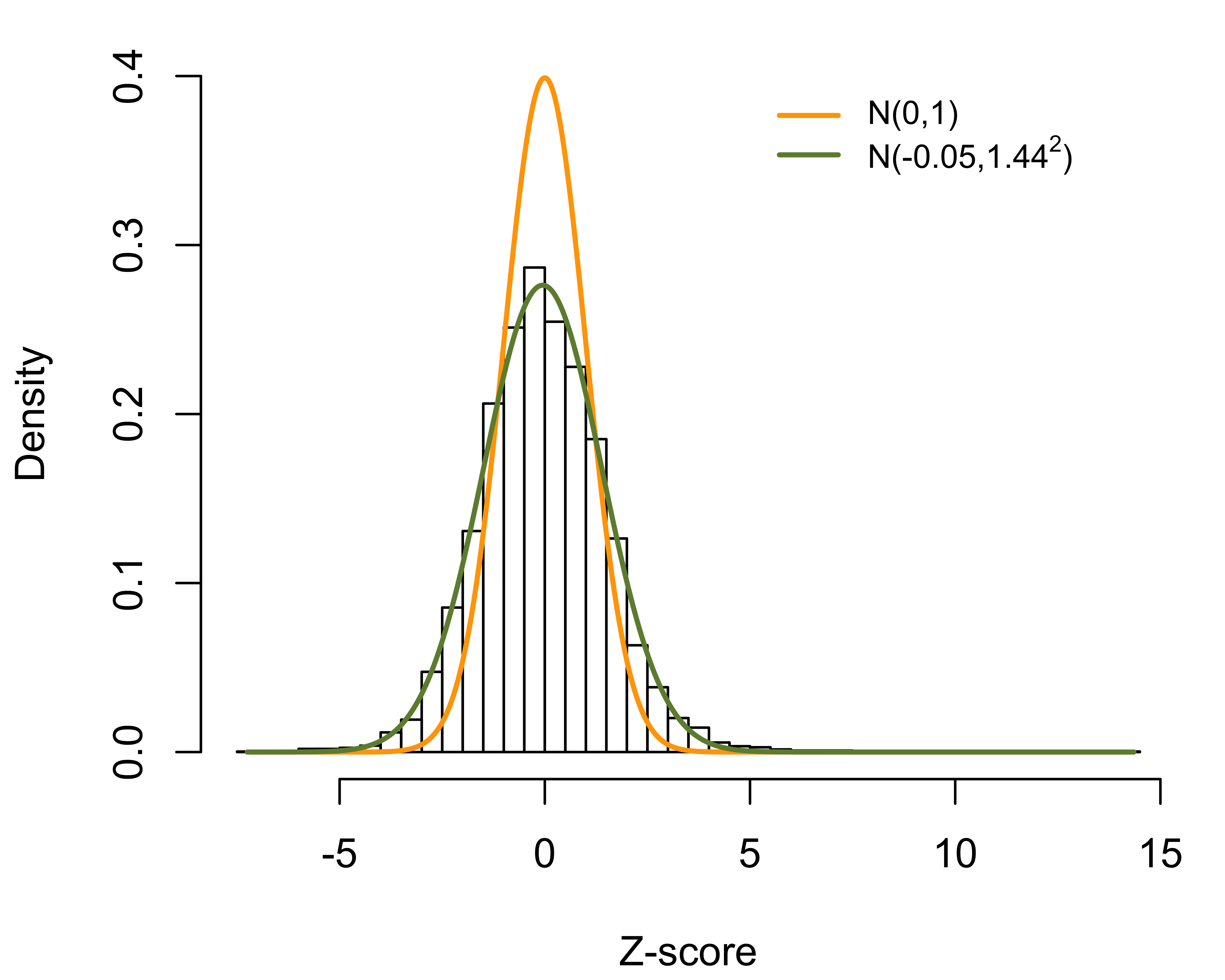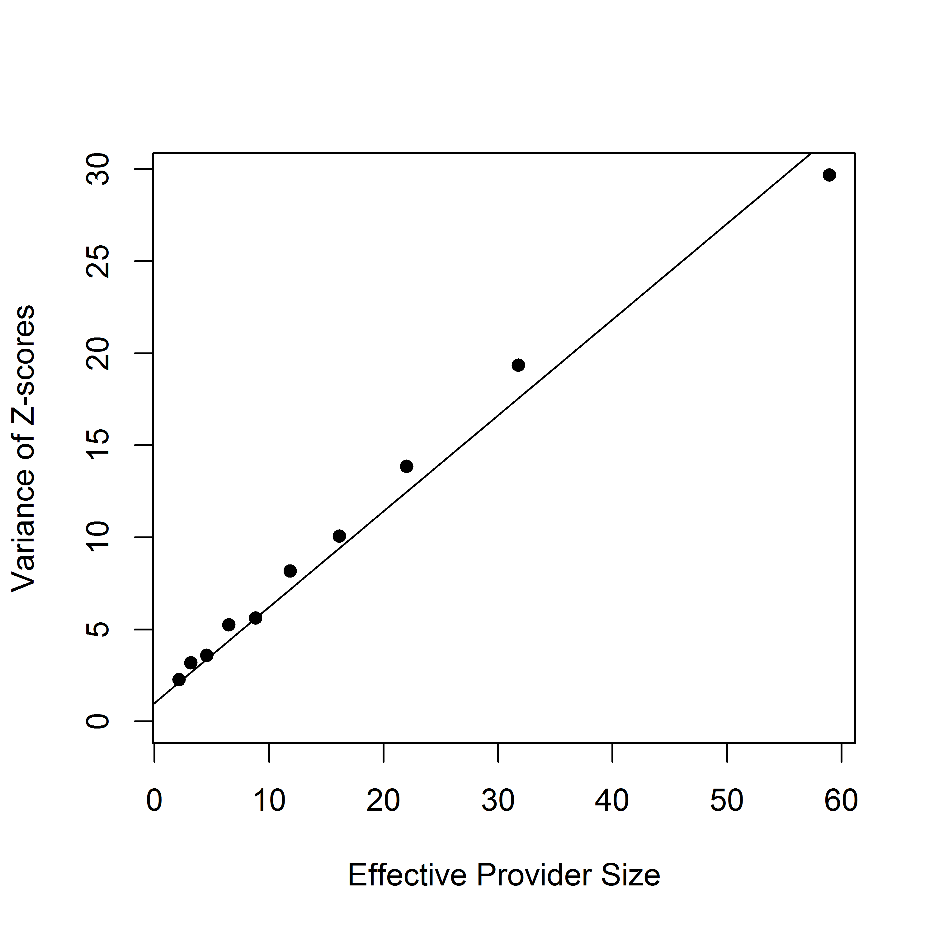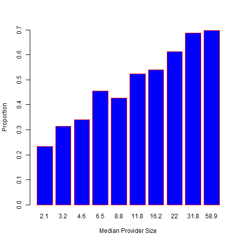Figure 2: Histogram of FE-based Z-scores for 6,363 dialysis facilities; overall and stratified by provider sizes..

​

2.2 Individualized Empirical Null

In practice, risk-adjustment is never perfect. Moreover, the existence of outlying providers will result in an over-estimation of the between-provider variation. The corresponding power is affected; likely to falsely forgive extreme outliers. To incorporate imperfect risk-adjustment and remove the effects of outlying providers, we consider an individualized two-group model. To illustrate the proposed method, we utilize the FE-based Z-scores, although the RE-based Z-scores can be applied as well. Suppose that $Z_{FE,i}$ is either from a null distribution with a prior probability $\pi_0$ or from a distribution of outliers with probability $\pi_1=1-\pi_0$. Assume the corresponding mixture density is given by a two-group model,

where the null density $f_{0,i}(z)$ is from a normal distribution with mean $\theta$ and variance $1+n_i \gamma$, and $f_{1,i}(z)$ is a density for outliers. Here $\gamma=\sigma_{\alpha}^2/\sigma_w^2$. To obtain robust estimates of $\theta$ and $\gamma$, we assume that the non-null density $f_{1,i}$ for the $i$th provider has support outside an interval

where $(\theta_0, \gamma_0)$ are initial estimates, and $c > 0$ is a specified number (e.g. 1.64). Let $I_0 = \{ i:\ Z_{FE, i} \in [A_i, B_i] \}$, $N_0 = |I_0|$, the cardinality of $I_0$, $N_1 = N - N_0$, and $\phi_{\theta,\gamma}(z|n_i)$ is the normal density with mean $\theta$ and variance $1+n_i\gamma$. Let $Q(\theta, \gamma)= \Phi(c)-\Phi(-c)$, where $\Phi(\cdot)$ is the cumulative distribution function of $N(0,1)$, be the probability that a null Z-score with sample size $n_i$ falls in the interval $[A_i, B_i]$. The likelihood is written as

One can numerically solve the optimization problem and find the maximum likelihood estimates, denoted as $\hat\pi_0$, $\hat\theta$ and $\hat\gamma$, respectively. The $i$th provider is flagged as worse than expected if $Z_{EN, i}>z_{p}$, where

Note that a robust M-estimation for heteroskedastic regression can be used to obtain the initial estimates of $(\mu_0, \gamma_0)$. This M-estimation is simple, but can give biased estimates of the variance, which motivated the proposed approach.

​

2.3 Frequentist Interpretation

Consider the provider-level sample mean $\bar{Y}_i$. Unconditionally on $\alpha_i$, denote the marginal mean of $\bar{Y}_i$ by $\mu_i=E(\bar{Y}_i)$. If provider $i$ comes from the null distribution, $\mu_i$ is an unbiased estimator of the population mean; i.e. $\mu_i=\mu$. Otherwise, $\mu_i \neq \mu$. Thus, $Z_{EN,i}$ can be considered as a test statistics for a null hypothesis $H_{0,i}~:~\mu_i=\mu$ against the alternative hypothesis $H_{1,i}~:~\mu_i>\mu$. The corresponding p-value is given by

​

2.4 Bayesian Interpretation

Under the linear model (2), the predictive distribution of $\bar{Y_i}$ is given by $N(\mu, \sigma_{\alpha}^2+\sigma_w^2/n_i)$. The predictive p-value for identifying extreme providers with mean larger than plausible

which leads to the same p-value as the frequentist interpretation.

​

2.5 Remarks

A simple approach (termed naive approach) is to directly estimate $\sigma_{\alpha}$ from a random effects model and standardize the Z-scores based on their marginal variance, so that the standardized Z-scores follow the standard normal distribution. However, the existence of outlying providers will result in an over-estimation of $\sigma_{\alpha}$, which will affect the power to identify extreme outliers. The idea of the empirical null was introduced in Efron in the context of multiple testing with a uniform null distribution. Kalbfleisch and Wolfe proposed using the empirical null distribution of the FE-based Z-scores to assess outlying providers. Specifically, a robust estimation technique is applied to obtain the mean and variance estimates of the FE-based Z-scores, which can then be used as reference in hypothesis testing. However, in application with provider profiling, the total variation for assessing provider effects and the distribution of the test statistics usually change with the provider’s sample size. This leads to individualized null distributions for the test-statistics, precluding the application of existing empirical null approaches. These concerns motivate the proposed individualized empirical null procedure.

​

3 Extensions to Non-Linear Models

​

3.1 Generalized Linear Models

The proposed approach accommodates many other types of outcomes.

Consider a generalized linear model

where $\pi(\cdot |\cdot)$ is the conditional density function, $\psi$ is a dispersion parameter, $a(\cdot)$ is a known function. Here $b(\cdot)$ is a specific known function with $\textrm{E}(Y_{ij} \mid \textbf{X}_{ij})=b'(\theta_{ij})$ and $\textrm{Var}(Y_{ij} \mid \textbf{X}_{ij})=a(\psi)b''(\theta_{ij})$. Here primes denote differentiation with respect to $\theta_{ij}$. We assume $\theta_{ij}=\mu+\alpha_i+\textbf{X}^T_{ij} \boldsymbol\beta$, where $\mu$ and $\boldsymbol\beta$ are estimated with great precision, which is justified given the large sample size for most profiling applications. The FE-based Z-score for a sharp null hypotheses $\alpha_i=0$ can be constructed via a score test statistic

where $\theta_{ij}^0=\mu+\textbf{X}^T_{ij} \boldsymbol\beta$. To incorporate unexplained variation between providers, we assume $\alpha_i \sim N(0, \sigma_{\alpha}^2)$. Applying a first-order Taylor expansion of $b'(\theta_{ij})$ and $b''(\theta_{ij})$ around $\theta_{ij}^0$, the marginal variance of $Z_{FE, i}$ can be approximated as

which is a linear function of $\sum_{j=1}^{n_i}b''(\theta_{ij}^0)$.

Example outcomes:

• Continuous outcome: under the linear model (2), we have $\sum_{j=1}^{n_i}b''(\theta_{ij}^0)=n_i$ and $a(\psi)=\sigma_w^2$.

• Binary Outcomes: let $Y_{ij}$ denote a binary outcome (e.g. hospital readmission within 30 days of index discharges). Consider a logistic model $\textrm{logit}(P_{ij})=\mu+ \alpha_i +\textbf{X}_{ij}^T\boldsymbol\beta$, where $P_{ij}=P(Y_{ij}=1|\alpha_i)$. Here $b(\cdot)=\log(1+\exp(\cdot))$, $a(\psi)=1$ and $b''(\theta_{ij}^0)=b'(\theta_{ij}^0)(1-b'(\theta_{ij}^0))$.

  Assuming $\alpha_i \sim N(0, \sigma_{\alpha}^2)$, the marginal variance of $Z_{FE, i}$ can be approximated as $1 + \tilde{n}_i\sigma_{\alpha}^2$, where $\tilde{n}_i=\sum_{j=1}^{n_i}\{b'(\theta_{ij}^0)(1-b'(\theta_{ij}^0))\}$. The proposed individualized empirical null approach can be easily applied based on $\tilde{n}_i$.

• Poisson outcomes: let $Y_{ij}$ be a Poisson outcome (e.g. ED visits) for the $j$th patient in the $i$th provider. Consider a Poisson model $\log(E(Y_{ij}))=\mu+ \alpha_i +\textbf{X}_{ij}^T\boldsymbol\beta$, with $b(\cdot)=\log(\cdot)$ and $b'(\theta_{ij}^0)=b''(\theta_{ij}^0)$. Assuming $\alpha_i \sim N(0, \sigma_{\alpha}^2)$, the approximate marginal variance of $Z_{FE,i}$ is given by $1 + \tilde{n}_i\sigma_{\alpha}^2$, where $\tilde{n}_i=\sum_{j=1}^{n_i}b'(\theta_{ij}^0)$.

​

3.2 Discrete Survival Models

In large-scale disease registries, ties in event times can be extremely numerous. Various approximation procedures, have been proposed for the partial likelihood to account for ties among failure times. However, when the ties are extremely numerous these approximation procedures can be seriously inadequate. As the proportion of ties expands, the bias of these approximations and the computational burden increase quickly, preventing the use of the standard partial likelihood approach. When the sample size is substantial and there is only a modest number of distinct event times, it becomes feasible to treat the baseline hazard at each event time as a parameter in the estimation algorithm, which also facilitates obtaining the absolute hazard. Moreover, in large-scale datasets, the number of unique failure times can be much smaller than the sample size. For example, in the national dialysis database, the time to event is rounded to the nearest days; thus, for 30 day readmission there would be numerous ties and only 30 discrete event times. This motivates the use of a discrete-time model.

Let $t_1, \ldots, t_h$ be the unique event times. Let $D_{i}$ denote the set of labels associated with individuals failing at time $t_i$. Let $C_{i}$ be the set of labels associated with individuals censored in time period $[t_i, t_{i+1})$. Let $R_{i}$ denote the at risk set at time $t_i$. Let $\textbf{X}_{l}=(X_{l1}, \ldots, X_{lP})^T$ be a $P$-dimensional covariate vector for subject $l$. Assume a general model, where the hazard at time $t_i$ for the $l$-th patient with covariate $\textbf{X}_{l}$ is denoted by $d\Lambda(t_i;\textbf{X}_{l})$. The likelihood function is given by

and the corresponding log-likelihood function is then given by

where $Y_{l}(t_i)$ is the at-risk indicator and $\delta_{l}(t_i)$ is the event indicator at $t_i$. Consider the formulation

where $f$ is a monotone and twice-differentiable function. The log-likelihood function of $\boldsymbol\gamma=(\gamma_1, \ldots, \gamma_h)^T$ and $\boldsymbol\beta=(\beta_1, \ldots, \beta_p)^T$ can be written

While other transformations are possible we will assume a log link that gives a discrete relative risk model, for which, In what follows, we consider two commonly used logit and log links, which correspond to the discrete logistic and the discrete relative risk models, respectively.
Consider the discrete logistic link function:

where $d\Lambda_{0}(t_i)=\exp(\gamma_i)$ is the baseline hazard at time $t_i$. $d\Lambda(t_i;\textbf{X}_{l})= d\Lambda_{0}(t_i) \exp\{\textbf{X}^\top_{l}(t_i)\},$ where $d\Lambda_{0}(t_i)=\exp(\gamma_i)$ is the baseline hazard at time $t_i$. The corresponding log-likelihood function is given by $\ell(\boldsymbol\gamma, \boldsymbol\theta) = \sum_{l=1}^{N} \ell_l(\boldsymbol\gamma, \boldsymbol\theta)$, which is additive, without the inner sum over the risk set, and hence is more conducive to utilize stochastic approximations. This model also facilitates obtaining the absolute hazards. Here

The log-likelihood function is

Alternatively, consider the log link $d\Lambda(t_i;\textbf{Z}_{l})= d\Lambda_{0}(t_i) \exp\{\textbf{Z}^\top_{l}\boldsymbol\beta(t_i)\}.$ The log-likelihood function is

Using B-splines, the log-likelihood function is

where $Y_{l}(t_i)$ is the at-risk indicator at $t_i$, $\delta_{l}(t_i)$ is the event indicator at $t_i$, $\boldsymbol\gamma=(\gamma_1, \ldots, \gamma_h)^T$, $\boldsymbol\theta$ and $\boldsymbol\Theta$ are the same as those defined in Aim 1a. The need is then to maximize this likelihood over both $\boldsymbol\gamma$ and $\boldsymbol\theta$.

The FE-based Z-score for a sharp null hypotheses $\alpha_i=0$ can be constructed via a score test statistics

where $h^0_{ijk}=h(\eta_k+\textbf{X}^T_{ij} \boldsymbol\beta)$. Note that in most profiling applications, $\eta_k$ and $\boldsymbol\beta$ are estimated with great precision, which is justified given the large sample size in the large-scale disease registries (e.g. an example is shown in Figure 11 with 541,769 discharges from 6,937 dialysis facilities). To incorporate unexplained variation between providers, we assume that $\alpha_i$ follows a random distribution with mean 0 and variance $\sigma_{\alpha}^2$. Applying a first-order Taylor expansion, the marginal variance of $Z_{FE, i}$ can be approximated as

​

4 Simulation

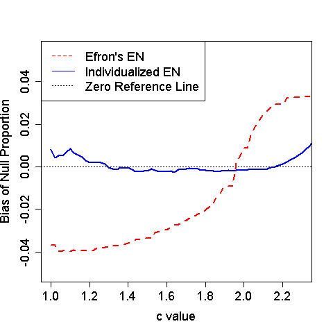
Figure 3: Estimated bias for null proportion with various values of $c$.

Binary outcomes were generated from a logistic regression with 600 providers and 10% of them being outlier. The null provider effect $\alpha_{i}$ was simulated from a standard normal distribution. The outlying provider effects were fixed at 3 times $\sigma_{\alpha}$. We varied the sample size such that one third of providers had 75, 150 and 300 patients, respectively. The tuning parameter $c$ in the truncated interval took values in $[1,2]$ by an increment of 0.02. Figure XX compares the bias of the estimated null proportion for various values of $c$. The proposed individualized empirical null provides sounds estimation. In contrast, the original empirical null ignores the fact that the test statistics for provider profiling changes with the provider’s sample size, and hence, leads to biased estimations of the null distribution and the proportion of null effects; when $c$ is small, the $\pi_0$ is under-estimated and the power to identify extreme providers will be reduced. When $c$ is large, the $\pi_0$ is over-estimated and the Type I error will be inflated.

​

5 Conclusion