​

Abstract

Large-scale time-to-event data derived from national disease registries arise rapidly in medical studies. Detecting and accounting for time-varying effects are particularly important, as time-varying effects have already been reported in the clinical literature. However, traditional methods of modeling time-varying survival models typically rely on expanding the original data in a repeated measurement format, which, even with a moderate sample size, usually leads to an intractably large working dataset. Consequently, the computational burden increases dramatically as the sample size grows, precluding the evaluation of time-varying effects in large-scale studies. On the other hand, to model time-varying effects for observations from national disease registries, small at-risk sets may arise due to rare comorbidities. Inverting the corresponding observed information matrix can be numerically unstable, especially near the end of the follow-up period, because of the censoring-caused sparsity. In view of these drawbacks, we propose a computationally efficient Kronecker product-based proximal algorithm, which enables us to extend existing methods of estimating time-varying effects for time-to-event data to a large-scale context.

Key words: Kidney Transplantation; Kronecker Product; Proximal Algorithm; Time-Varying Effects.

​

1 Introduction

The time-varying effects model is a flexible and powerful tool for modeling the time-varying covariate effects. However, in survival analysis, its computational burden increases quickly as the number of observations grows. Traditional methods that perform well for small-sized data do not scale to large-scale data. Analysis of large databases derived from national disease registries studies defy any existing statistical methods and software.

Our endeavor here is motivated by the study of end-stage renal disease (ESRD), which represents 6.7% of the entire Medicare budget (Saran2018). Kidney transplantation is the preferred treatment for ESRD. However, despite aggressive efforts to increase the number of kidney donors, the demand far exceeds the supply. In 2016, the kidney transplant waiting list had 83,978 candidates, with fewer than 16% of eligible patients likely to receive a transplant (Saran et al., 2018). To optimize treatment strategies for ESRD patients, an important aspect is that different patients may respond to transplantation differently and it is crucial to understand why the outcome is worse for certain patients. To achieve this goal, detecting and accounting for time-varying effects are particularly important in the context of ESRD studies, as time-varying effects have already been reported in the clinical literature (Kalantar-Zadeh, 2005, Dekker et al., 2008, Englesbe et al., 2012). These time-varying associations make it difficult to use the proportional hazards model in ESRD studies, as ignoring the time-varying nature of covariate effects may obscure true risk factors.

A wide variety of methods have been studied for time-varying effects in survival analysis. Zucker et al. (1990) utilized a penalized partial likelihood approach. Gray (1992) proposed using fixed knots spline functions. He et al. (2017) considered a quasi-Newton-based approach. Some recent studies Yan et al. (2012) have proposed selection of time-varying effects using penalized methods such as adaptive Lasso (Zou, 2006, Zhang and Lu, 2017). However, in large-scale studies, these algorithms, which involve iterative computation and inversion of the observed information matrix, can easily overwhelms a computer with a 32G memory. Moreover, to estimate the time-varying effects, one may represent the coefficients using basis expansions such as B-splines. Thus, the parameter vector carries block structures, for which extra parameters are created and the computational burden increases quickly as the number of predictors grows. Furthermore, in our motivating example, small at-risk sets may arise due to rare comorbidities. The inversion of the observed information matrix can be numerically unstable, especially in the right-tail of the follow-up period, because the data tends to be sparse there due to censoring.

To illustrate this issue, we generated five binary covariates with specified frequencies between 0.05 and 0.2. Detailed simulation set-ups are provided in Section 2 of Section 3. As shown in Figures 1a and 1b, the classical Newton approach faces serious limitations with slow convergence and unstable estimations. In particular, to estimate time-varying effects, traditional methods rely on an expansion of the original dataset in a repeated measurement format, where the time is divided into small intervals of a single event. Within each interval, the covariate values and outcomes for at-risk subjects are stacked to a large working dataset, which becomes infeasible for large sample sizes. Moreover, when the at-risk sets are small, the classical Newton approach introduces large estimation biases. In contrast, our proposed approach is computationally efficient and substantially improves the estimation error.

The remainder of this article is organized as follows: In Section 2 we briefly review some preliminary notations and then develop a Kronecker product-based proximal algorithm. In Section 3 we evaluate the practical utility of the proposed method via simulation studies. In Section 4 we apply the proposed method to analyze the national kidney transplantation data. We conclude the article with a brief discussion in Section 5.

​

2 Method

​

2.1 Time-Varying Effect Model

Let $D_{i}$ denote the time lag from transplantation to death and $C_{i}$ be the censoring time for patient $i$, $i=1,\ldots, n$. Here $n_j$ is the sample size. The observed time is $T_{i} = \min\{D_{i},C_{i}\}$, and the death indicator is given by $\delta_{i} = I(D_{i} \leq C_{i})$. Let $\textbf{X}_{i}=(X_{i1}, \ldots, X_{iP})^T$ be a $P$-dimensional covariate vector. We assume that $D_{i}$ is independent from $C_{i}$ given $\textbf{X}_{i}$.

Consider the hazard function

where $\lambda_{0}(t)$ is the baseline hazard. To estimate the time-varying coefficients ${\boldsymbol\beta}(t)=\{\beta_{1}(t),\ldots, \beta_{P}(t)\}$, we span $\boldsymbol\beta(\cdot)$ by a set of cubic B-splines defined on a given number of knots:

where $\textbf{B}(t)=\{B_1(t), \ldots, B_K(t)\}^T$ forms a basis, $K$ is the number of basis functions, and $\boldsymbol\theta*{p}=(\theta_{p1}, \ldots, \theta{pK})^T$ is a vector of coefficients with $\theta_{pk}$ being the coefficient for the $k$-th basis of the $p$-th covariate. With a length-$PK$ parameter vector $\boldsymbol\theta=vec(\boldsymbol\Theta)$, the vectorization of the coefficient matrix $\boldsymbol\Theta=(\boldsymbol\theta_{1}, \ldots, \boldsymbol\theta_{P})^T$ by row, the log-partial likelihood function is

where $R_{i}=\{i': 1 \leq i' \leq n, ~ T_{i'}\geq T_{i}\}$ is the at-risk set. That $\boldsymbol\theta$ has $P$ “blocks” of subvectors, i.e. $\boldsymbol\theta_{p}, p=1, \ldots,P,$ each corresponding to a covariate, will inform the development of our proposed block-wise steepest ascent algorithm.

​

2.2 Newton’s Approach

When both $N$ and $P$ are moderate, maximization of $(1)$ can be achieved by a Newton approach, which requires computation of the gradient and Hessian matrix, given by $\triangledown \ell(\boldsymbol\theta)= \sum_{i} \Psi_{i}(\boldsymbol\theta)$ and

respectively. Here $\otimes$ is the Kronecker product, and

where

for $r=0, 1,2$. For a column vector $\textbf{v}$, $\textbf{v}^{\otimes 0} =1$, $\textbf{v}^{\otimes 1} =\textbf{v}$ and $\textbf{v}^{\otimes 2}=\textbf{v}\textbf{v}^T$.

​

2.3 Stratified Time-Varying Effect Model

When different facilities are present, we can extend the model to stratified version. Let $D_{ij}$ denote the time lag from transplantation to death and $C_{ij}$ be the censoring time for patient $i$ in center $j$, $i=1,\ldots, n_j$, and $j=1, \ldots, J$. Here $n_j$ is the sample size in center $j$, and $J$ is the number of centers. The total number of patients is $N=\sum_{j=1}^Jn_j$, the observed time is $T_{ij} = \min\{D_{ij},C_{ij}\}$, and the death indicator is given by $\delta_{ij} = I(D_{ij} \leq C_{ij})$. Let $\textbf{X}_{ij}=(X_{ij1}, \ldots, X_{ijP})^T$ be a $P$-dimensional covariate vector. We assume that $D_{ij}$ is independent from $C_{ij}$ given $\textbf{X}_{ij}$.

Consider a stratum-specific hazard function

where $\lambda_{0j}(t)$ is the baseline hazard for stratum $j$. To estimate the time-varying coefficients ${\boldsymbol\beta}(t)=\{\beta_{1}(t),\ldots, \beta_{P}(t)\}$, we span $\boldsymbol\beta(\cdot)$ by a set of cubic B-splines defined on a given number of knots:

where $\textbf{B}(t)=\{B_1(t), \ldots, B_K(t)\}^T$ forms a basis, $K$ is the number of basis functions, and $\boldsymbol\theta_{p}=(\theta_{p1}, \ldots, \theta_{pK})^T$ is a vector of coefficients with $\theta_{pk}$ being the coefficient for the $k$-th basis of the $p$-th covariate. With a length-$PK$ parameter vector $\boldsymbol\theta=vec(\boldsymbol\Theta)$, the vectorization of the coefficient matrix $\boldsymbol\Theta=(\boldsymbol\theta_{1}, \ldots, \boldsymbol\theta_{P})^T$ by row, the log-partial likelihood function is

where $R_{ij}=\{i': 1 \leq i' \leq n_j, ~ T_{i' j}\geq T_{ij}\}$ is the at-risk set for stratum $j$. That $\boldsymbol\theta$ has $P$ “blocks” of subvectors, i.e. $\boldsymbol\theta_{p}, p=1, \ldots,P,$ each corresponding to a covariate, will inform the development of our proposed block-wise steepest ascent algorithm.

​

2.4 Newton’s Approach for Stratified Model

When both $N$ and $P$ are moderate, maximization of $(6)$ can be achieved by a Newton approach, which requires computation of the gradient and Hessian matrix, given by $\triangledown \ell(\boldsymbol\theta)=\sum_{j} \sum_{i} \Psi_{ij}(\boldsymbol\theta)$ and

respectively. Here $\otimes$ is the Kronecker product, and

where

for $r=0, 1,2$. For a column vector $\textbf{v}$, $\textbf{v}^{\otimes 0} =1$, $\textbf{v}^{\otimes 1} =\textbf{v}$ and $\textbf{v}^{\otimes 2}=\textbf{v}\textbf{v}^T$.

​

2.4.1 Backtracking Linesearch

The step size plays an important role in terms of estimation accuracy and computational efficiency. Parikh et al. (2014) proposed the backtracking linesearch to adjust the step size. The Newton increment $\nabla \ell(\boldsymbol\gamma^{(m)})^\top \boldsymbol\mu^{(m)}$ is defined in the book. This backtracking linesearch, uses Armijo condition, which requires a sufficient increase in $\ell$ proportional to step length $\nu$ and Newton increment before the line search is terminated. Detailed discussion can be found in.

When binary predictors with extremely low frequency are present, calculation of the second order derivative has some issues. In that case, the Newton increment presents extreme values, leading to huge bias. We provided a way of limiting the step size in such cases. Instead of using the Newton increment in step, we use a fixed value of 1. This method is referred as “static” in our function. Since it moves slower, usually it can not achieve maximum likelihood estimator, leading to biased estimation. Specifically, it consitutes a practical implementation of the Armijo-Goldstein conditions

​

2.4.2 Stopping Criteria

The convergence criteria also plays an important role here. We define $(\ell^{(m)}-\ell^{(m-1)})/(\ell^{(m)}-\ell^{(0)})$ as the relative change of the log-partial likelihood, where $m$ denotes the $m_{th}$ step of the algorithm. When it’s smaller than a certain threshold, we stop the algorithm. $\textit{tol}$ is the variable determining the convergence threshold. The default threshold is set as $10^{-6}$. This is a relatively conservative way of stopping the algorithm, leading to convergence in most cases.

We also provide other simple choices of stopping criteria in our package. “ratch” is the default way talked above. “relch” defines the relative change of the log-partial likelihood as $(\ell^{(m)}-\ell^{(m-1)})/(\ell^{(m)})$, which makes it easier to converge. “incre” would stop the algorithm when the half of the Newton increment is less than the threshold. “all” won’t stop the algorithm until “ratch”, “relch” and “incre” is met. This is the most conservative way of stopping the algorithm.

​

2.5 Proximal Newton—Raphson

Wu et al., (2022) showed the superiority of using proximal Newton’s algorithm. By adding a small term to the Diagonal of the $\nabla^2 \ell(\boldsymbol\theta^{(m)})$ matrix, we can get more stable estimation with faster convergence.

​

2.6 Penalized Newton’s Method

The proximal Newton can help improve the estimation when the origional hessian matrix is very close to a singular one, which may often occur in the setting of time-varying effects, however, over-fitting issue still exists. We further improve the estimation by introducing the penalty. The basic idea of penalization is to control the model’s smoothness by adding a ‘wiggliness’ penalty to the fitting objective. Rather than fitting the non-proportional hazards model by maximizing original log-partial likelihood, it could be fitted by maximizing

We have different choices of $P_\lambda(\boldsymbol\theta)$. Potential choices are to use P-splines, and discrete penalties. Detailed discussions are provided below.

​

2.6.1 P-spline

The P-splines are low rank smoothers using a B-spline basis, usually defined on evenly spaced knots, with a difference penalty applied directly to the parameters $\theta_{pk}$, to control function wiggliness. When we set standard cubic B-spline basis functions, the penalty function used for $\beta_p$ will be

Therefore the summation term measures wiggliness as a sum of squared second differencess of the function at the knots (which crudely approximates the integrated squared second derivative penalty used in cubic spline smoothing). When $\beta_p$ is very wiggly the penalty will take high values and when $f$ is ‘smooth’ the penalty will be low. If $\beta_p$ is a straight line, then the penalty is actually zero.

It is straight forward to express the penalty as a quadratic form, $\boldsymbol\theta^T\textbf{S}\boldsymbol\theta$, in this basis coefficients:

Hence the penalized fitting problem is to maximize

with respect to $\boldsymbol\theta$. The problem of evaluating smoothness for the model turns to estimating the smoothing parameter $\lambda$. But before addressing $\lambda$ estimation, consider $\boldsymbol\beta$ estimation give $\lambda$.

P-splines have three properties that make them very popular as reduced rank smoothers. First, the basis and penalty are sparse, enabling efficient computation; Second, it is possible to flexibly ‘mix-and-match’ the order of B-spline basis and penalty, rather than the order of penalty controlling the order of the basis; Third, it is very easy to set up the B-spline basis functions and penalties. However, the simplicity is somewhat diminished when uneven knot spacing is required.

​

2.6.2 Smoothing-spline

The reduced rank spline smoothers with derivative based penalties can be set up almost as easily, while retaining the sparsity of the basis and penalty and the ability to mix-and-match the orders of spline basis functions and penalties.

We denote the B-spline basis as of order $m_1$, and $m_1 = 3$ denotes a cubic spline. Associated with the spline will be a derivative based penalty

where $\boldsymbol\beta^{[m_2]}(t)$ denotes the $m_2^{th}$ derivative of $\boldsymbol\beta$ with respect to $t$. It is assumed that $m_2 \leq m_1$, otherwise it makes no sense that the penalty is formulated in terms of a derivative that is not properly defined for the basis functions. Similarly, $P_{\lambda}$ can be written as $\boldsymbol\theta^T\textbf{S}\boldsymbol\theta$ where $\textbf{S}$ is a band diagonal matrix of known coefficients.

The derivation of the algorithm is quite straightforward. Given the basis expansion we have that

However by construction $B_{m_1,i}^{[m_2]}(x)$ is made up of order $p = m_1 - m_2$ polynomial segments. So we are really interested in integrals of the form

for some polynomial coefficients $a_i$ and $d_j$. The polynomial coefficients are the solution obtained by evaluating $B_{m_1,i}^{[m_2]}(x)$ at $p+1$ points spaced evenly from $x_l$ to $x_{l+1}$, to obtain a vector of evalutated derivatives, $\mathbf{g}_a$, and then solving $\textbf{P}\mathbf{a} = \mathbf{g}_a$ ($\mathbf{d}$ is obtained from $\mathbf{g}_d$ similarly). Then $S_{ij} = \sum_lS_{ijl}$.

Given that $\int_{-1}^{1}x^qdx = (1+(-1)^q)/(q+1)$ it is clear that $S_{ijl} = h_l\mathbf{a}^T\textbf{H}\mathbf{d}/2$ where $H_{ij} = (1+(-1)^{i+j-2})/(i+j-1)$($i$ and $j$ start at 1). In terms of the evaluated gradient vectors,

The $\textbf{G}$ matrix simply maps $\boldsymbol\beta$ to the concatenated (and duplicate deleted) gradient vectors for all intervals, while $\textbf{W}$ is just the overlapping-block diagonal matrix with blocks given by $h_l\textbf{P}^{-T}\textbf{H}\textbf{P}^{-1}/2$, hence $S_{ij} = \textbf{G}_i^T\textbf{W}\textbf{G}_j$, where $\textbf{G}_i$ is the $i^{th}$ row of $\textbf{G}$. The simpilicty of the algorithm rests on the ease with which $\textbf{G}$ and $\textbf{W}$ can be computed.

Specifically, $m_1 = 3$ denotes the cubic spline, and $m_2 = 2$ denotes the quadratic spline. Cubic B spline penalizing the second order derivative, reducing to a linear term. Quadratic B spline penalizing first order derivative, reducing to constant, which is also the same for Cubic B spline penalizing first order derivative.

We utilized splineDesign function provided in $\textit{splines}$ package to construct the spline functions. When constructing B-spline, we only need to specify the interior knots. Let the number of interior knots be K. The dimension of returned matrix is N * (K+degree+1).

Gray (1992) suggests using quadratic B splines penalizing the first order derivative since cubic splines tend to be unstable in the right tail of the distribution because the sparsity of data due to censoring. We find that using cubic B-spline penalizing the first order derivative are quite unstable, not suitable for our setting. Cubic B-spline penalizing the second order derivative gives similar estimation with higher variance compared with using quadratic B-spline penalizing the first order derivative.

​

2.6.3 Penalized Newton’s Method

We now derive the Newton-Raphson algorithm for maximizing the penalized log-partial likelihood $\ell_p(\boldsymbol\theta)$:

Straightforward calculations show that the gradient and Hessian matrix required by the Newton’s approach is given by $\triangledown \ell_p(\boldsymbol\theta)=\triangledown \ell(\boldsymbol\theta) - \lambda\boldsymbol\theta$ and

respectively, where $\triangledown \ell(\boldsymbol\theta)$ and $\triangledown^2 \ell(\boldsymbol\theta)$ is the same as in section 2.2.

In terms of implementation, we simply replace the $\triangledown \ell(\boldsymbol\theta)$ and $\triangledown^2 \ell(\boldsymbol\theta)$ by the $\triangledown \ell_p(\boldsymbol\theta)$ and $\triangledown^2 \ell_p(\boldsymbol\theta)$ in Algorithm 1.

​

2.6.4 Selection of Smoothing Parameter

In order to select the proper smoothing parameter, we utilize the idea of information criteria. We provide four different information criteria to select the optimal smooting parameter $\lambda$. Generally, $\textit{mAIC}, \textit{TIC}$ and $\textit{GIC}$ selects similar parameters and the difference of resulting estimations are barely noticable.

We define the Information Criteria as:

Generally, $\textit{mAIC}$ and $\textit{GIC}$ select similar $\lambda$, while $\textit{TIC}$ tends to select slightly smaller values. In terms of estimation results, the effects of smoothing parameters chosen by the three different criteria are barely noticeable.

We also borrowed the definition of ‘degrees of freedom’ from Hastie (1990) and conducted one Information Criteria:

Generally Hastie selects larger smoothing parameters. The effect is also small in terms of estimation.

​

2.7 Cross Validation

We also provided cross-validation to select the best smoothing parameter. Ching et al. (2018)

​

2.8 Testing of time-varying effects

To test whether the effects are time-varying, we use the constant property of B-splines, that is, if $\theta_{p1}=\cdots=\theta_{pK},$ the corresponding covariate effect is time-independent. Specify a matrix $\textbf{C}_p$ such that $\textbf{C}_p\boldsymbol\theta=\textbf{0}$ corresponds to the contrast that $\theta_{p1}=\cdots=\theta_{pK}$. Following , a Wald statistic can be constructed by

where $\boldsymbol{\widehat\theta}$ is obtained through the proposed BSA.

In the SEER database with large $N$, computation of the observed information matrix is infeasible as discussed in Section 2.2, though gradients are easier to compute. We consider a modified statistic

where $\textbf{V}(\boldsymbol{\widehat{\theta}})=\sum_{i=1}^{n}\Psi_{i} (\boldsymbol{\widehat\theta}) \Psi_{i} (\boldsymbol{\widehat\theta})^T$ is an approximation of the empirical information matrix, with $\Psi_{i}$ defined in. Under the null hypothesis that the effect is time-independent, $S_p$ is asymptotically chi-square distributed with $K-1$ degrees of freedom. % In some biomedical studies, the events of subjects within the same strata may be correlated, resulting in clustered data. For example, in familial studies, individuals within a family may be correlated due to shared genetic factors. To incorporate potential correlations among patients within strata, a robust inference procedure can be adopted.

​

3 Example implementation in R with simulation studies

​

3.1 Data set

We generate a single data set with the sample size equal to 5,000. Death times were generated from an exponential model with a contant baseline hazard 0.5. We considered 5 predictors sampled from a multivariate normal distribution with mean = 0, the variance = 1, and the covariance structure followed an $\textbf{AR}(1)$ correlation with an auto-correlation parameter 0.6. The true time-varying coefficient curves are $\boldsymbol\beta(t) = [1, \exp(-3t/2), -1, -(t/3)^2\exp(t/2), sin(3\pi t/4)]^T$. Censoring times were generated from a Uniform (0,3) distribution. Observed times were the minimum of the failure and censoring time pairs.

​

3.2 R environment and pacakages

The code was tested using R version 4.1.2 and RStudio version 2022.02.0. R packages $\textit{mvtnorm}$ (Genz et al., 2021) and $\textit{splines}$ were used directly. $\textit{Rcpp}$ and $\textit{RcppArmadillo}$ is utilized to improve computationtal speed. Additionaly the $\textit{survival}$ package is used for simulation.

​

3.3 Preliminaries

​

3.3.1 Install and load packages

For all examples in this tutorial, we used the R pacakge $\textit{surtvp}$ to estimate time-varying effects models. We have assumed that readers have some elementary familiarity with R, including how to install packages and manage data sets. The $\textit{surtvp}$ R package is available from Github at https://github.com/umich-biostatistics/PenalizedNR and it can be easily installed using $\textit{devtools}$ package as follows,

install.packages("devtools")
devtools::install_github("umich-biostatistics/PenalizedNR")

Then the $\textit{surtvp}$ package can be loaded as follows:

library(surtvp)

​

3.3.2 Data exploration

The data set in section 3.3.1 is included in the $\textit{surtvp}$ as a built-in data set. The data set was named $\textit{simulData}$ and its information can be viewed by

> str(simulData)

'data.frame': 5000 obs. of 7 variables:
$ event: num 1 1 1 0 0 1 1 1 0 1 ...
$ time : num 0 0.000405 0.000552 0.00073 0.000935 ...
$ z1 : num 0 0 0 0 0 1 1 0 0 0 ...
$ z2 : num 0 0 0 0 0 1 0 0 0 0 ...
$ z3 : num 0 0 0 0 0 0 0 0 0 0 ...
$ z4 : num 0 0 0 0 0 1 0 0 0 0 ...
$ z5 : num 0 0 0 0 0 0 0 0 0 0 ...

​

3.4 Selected methods

In this section, an overview of NR’s method and penalized NR’s method are given. The overview is followed by appplying the methods in a step-by-step tutorial using the $\textit{surtvp}$ R package.

​

3.4.1 Newton’s method

The surtvep() function requires similar inputs to the familiar coxph() from the package $\textit{survival}$.

surtvep(formula, data = matrix(), ...)

The input formula has the form Surv(time, event) ~ variable1 + variable2. The input data is in matrix form or a data frame. Additional parameters can be set for the Newton’s method: $\textit{nsplines}$, $\textit{degree}$, $\textit{method}$, $\textit{btr}$, $\textit{tol}$, $\textit{iter.max}$, $\textit{stop}$, $\textit{ties}$, $\textit{parallel}$, and $\textit{threads}$.

$\textit{nsplines}$ determines the number of basis functions for spanning parameter space. The default value is 10. $\textit{degree}$ has two potential choices. $\textit{degree} = 3$ uses cubic spline, and $\textit{degree} = 2$ uses quadratic spline. Generally, the estimation plots are more wiggled with more number of basis function. $\textit{method}$ has two options: “Newton” and “ProxN”, implementing the algorithm (1) and (2) correspondingly. $\textit{btr}$ has the default value of “dynamic”, choosing the step size based on algorithm (1). When binary predictors with extremely low frequency are present, calculation of the second order derivative has some issues. “static” can be used instead which takes a very small fixed step size. $\textit{tol}$ determines the threshold when the algorithm stops with the default value of $10^{-6}$. When the relative change of the log-partial likelihood is smaller than $\textit{tol}$, we stop the algorithm. $\textit{iter.max}$ is used to determine the maximum number of iterations to run the algorithm, default value is 20. $\textit{ties}$ allows to use Breslow approximation with the value of “Breslow” to speed up the algorithm when data with ties are present. The default value is “none"". $\textit{parallel}$ and $\textit{threads}$ are parameters related to parallel computation to improve computational speed. When $\textit{parallel}$ is set as “TRUE”, integer $\textit{threads}$ is the number of threads used to run the algorithm. Detailed examples are present below.

This is a simple example estimating the $\textit{simulData}$.

> fit1 <- surtvep(Surv(time, event)~., data = simulData)

Iter 1: Obj fun = -3.8152115; Stopping crit = 1.0000000e+00;
Iter 2: Obj fun = -3.7976069; Stopping crit = 3.5946947e-01;
Iter 3: Obj fun = -3.7967319; Stopping crit = 1.7553267e-02;
Iter 4: Obj fun = -3.7965909; Stopping crit = 2.8199439e-03;
Iter 5: Obj fun = -3.7965606; Stopping crit = 6.0619164e-04;
Iter 6: Obj fun = -3.7965587; Stopping crit = 3.7533135e-05;
Iter 7: Obj fun = -3.7965587; Stopping crit = 2.0119737e-07;
Iter 8: Obj fun = -3.7965587; Stopping crit = 6.5341279e-12;
Algorithm converged after 8 iterations.

The estimation results can be viewed by the plot() function.

plot(fit1)

Figure 1 shows the estimation plots of constant covariate and time-varying covariate using different number of basis function. The red curves are 95% confidence interval. Larger number of basis functions add more “wiggleness” to the estimation.

(a) constant coefficient 10 knots	(b) time-varying coefficient 10 knots

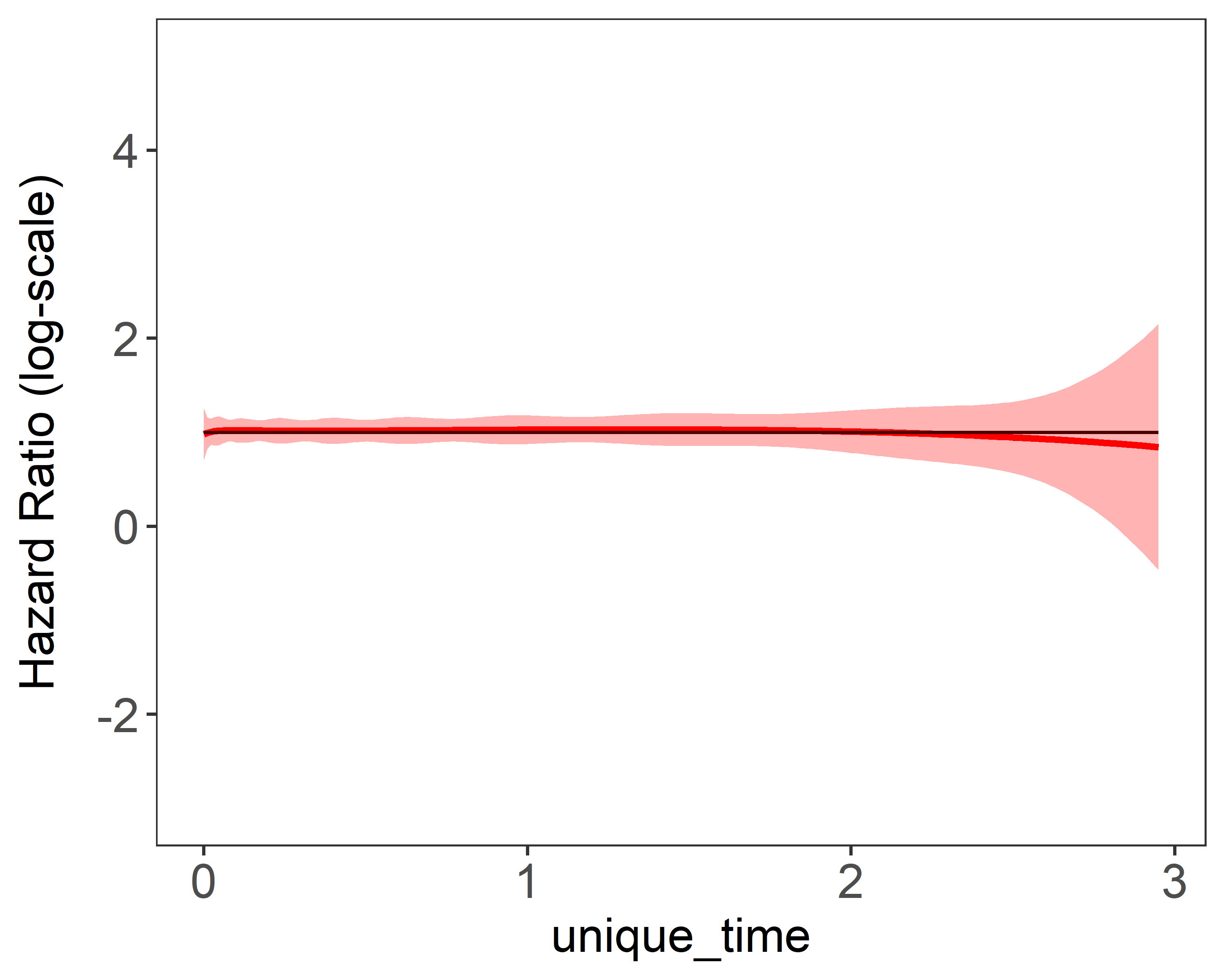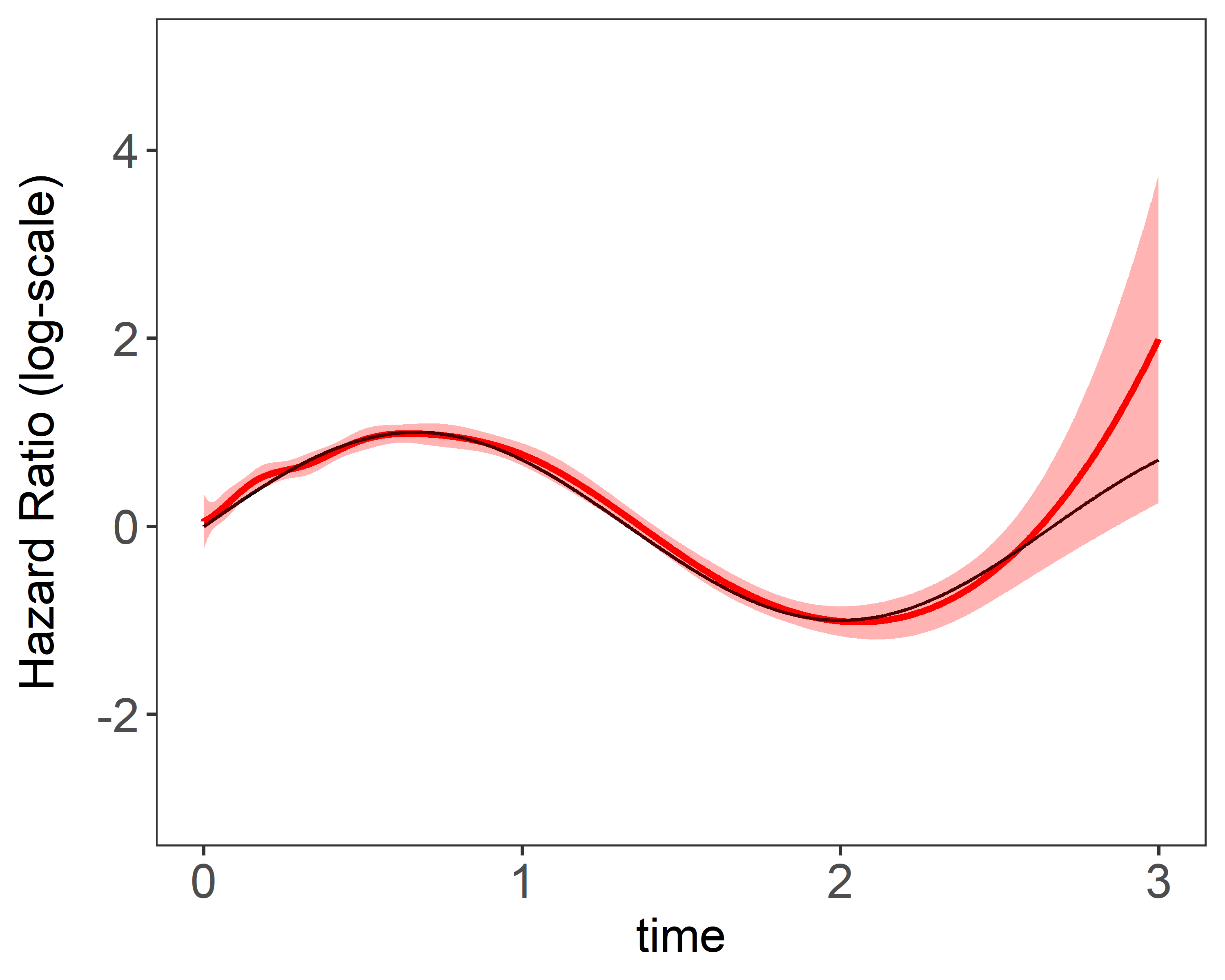Figure 1: Estimation plots produced by plot(fit)}. 1 single data replicate was generated with a sample size of 5,000. The model is fitted with a fixed number $K=10$ basis functions. True values were $\boldsymbol\beta(t) = 1$ and $\boldsymbol\beta(t) = sin(3\pi t/4)$

The speed up brought by the paralleled computation by can compared by implementing the following codes:

fit2 <- surtvep(Surv(time, event)~., data = simulData, parallel = False)

fit3 <- surtvep(Surv(time, event)~., data = simulData, parallel = TRUE, threads = 4)

​

3.4.2 Penalized Newton’s method

In order to add penalty to the penalized Newton’s method, three additional parameters can be added. $\textit{lambda}$, $\textit{spline}$ and $\textit{IC}$. $\textit{lambda}$ requires a sequence of input values as the smoothing parameter. $\textit{spline}$ is the type of penalty spline used to fit the algorithm. “Smooth-spline” and “P-spline” corresponds to Smoothing spline and P-spline separately. $\textit{IC}$ specifies the information criterion to be used for smoothing parameter selection. “mAIC”, “TIC”, “GIC” and “all” are valid inputs, returning parameter chosen by $\textit{mAIC}$, $\textit{TIC}$, $\textit{GIC}$ and all the results correspondingly.

fit.spline <- surtvep(Surv(time, event) ~ ., data = simulData,
                      lambda = c(0 : 100),
                      spline = "Smooth-spline",
                      IC = "all",
                      parallel = TRUE, threads = 4)

The resulting estimation plot with smoothing parameter chosen by $\textit{TIC}$ can be viewed by

plot(spline, IC = "TIC")

Figure 2 shows the results of estimation plots using NR’s method and penalized NR’s method with smoothing parameters selected by $\textit{TIC}$. Penalization suggested more number of knots will be to get better estimation without worrying about unstableness.

(a) constant coefficient 10 knots	(b) time-varying coefficient 10 knots

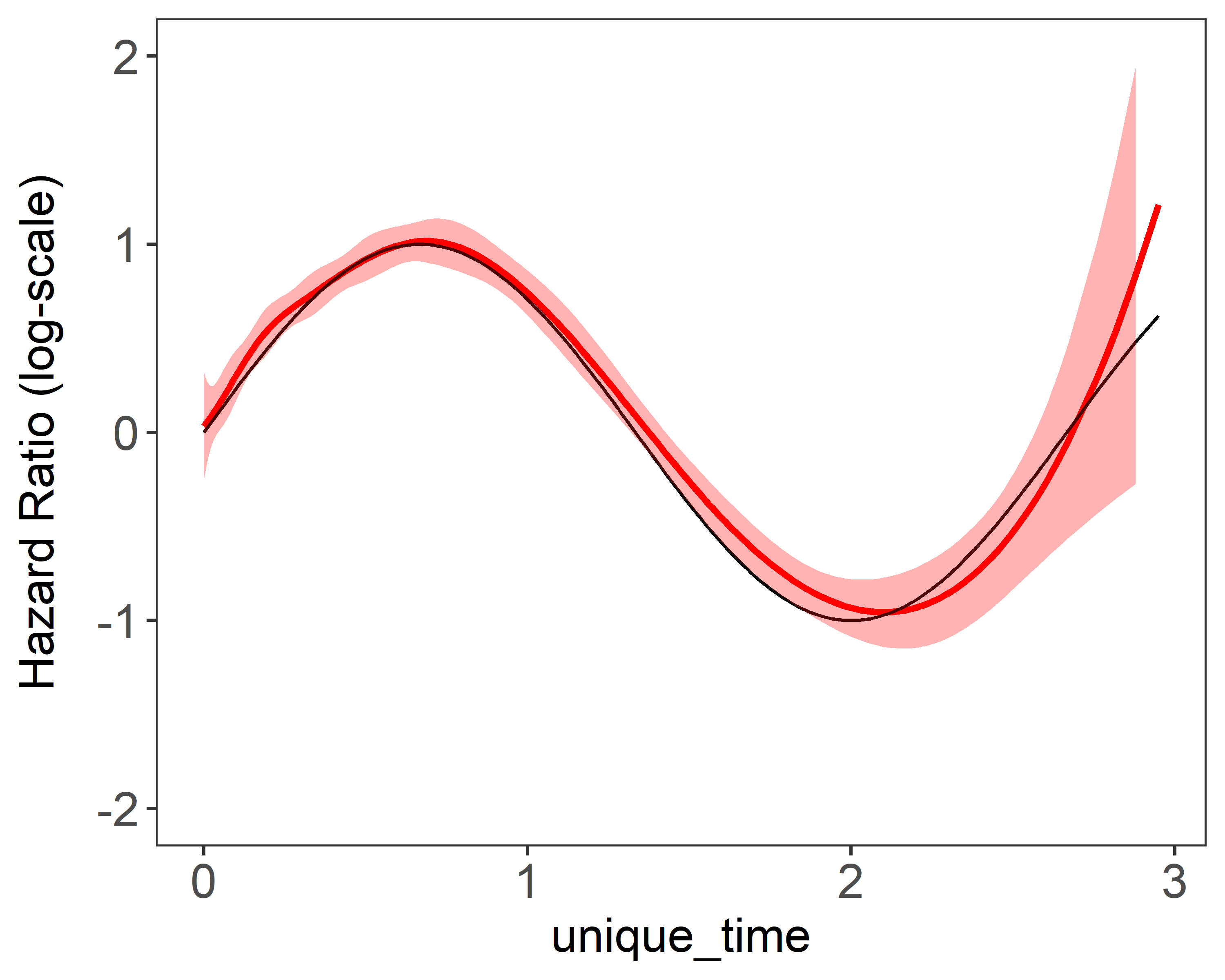Figure 2 Single estimation plots produced by plot(fit). 1 single data replicate was generated with a sample size of 5,000. The model is fitted with a fixed number of $K=6$ and $K=10$ basis functions. True values were $\boldsymbol\beta(t) = 1$ and $\boldsymbol\beta(t) = sin(3\pi t/4)$.

​

4 Data Example

This data example studies the risk-factors for mortality in different types of cancers using data from the National Cancer Institute Surveillance, Epidemiology, and End Results (SEER) Program. Mortality rates among cancer patients vary greatly, which merits special scrutiny of the associated risk factors. Baseline covariates obtained from the SEER Program are frequently used for risk adjustment, and the Cox proportional hazards model has been commonly used. However, researchers have observed that the covariate effects are often not constant over time. These time-varying associations make it difficult to use the proportional hazards model in cancer studies, as ignoring the time-varying nature of covariate effects may obscure true risk factors with corresponding implications for risk prediction, treatment development and health-care guidelines.

Since SEER data sets’ observation time are tied in months, we use Breslow approximation to improve estimation and speed. We compare the proximal newton’s algorithm and penalized Newton’s algorithm with parameters chosen by $\textit{TIC}$. The implementation of Colon are taken as an example:

fit.spline <- surtvep(Surv(time, event) ~ ., data = SEERcolon,
                     lambda = seq(),
                     spline = "Smooth-spline",
                     IC = "all",
                     parallel = TRUE, threads = 4)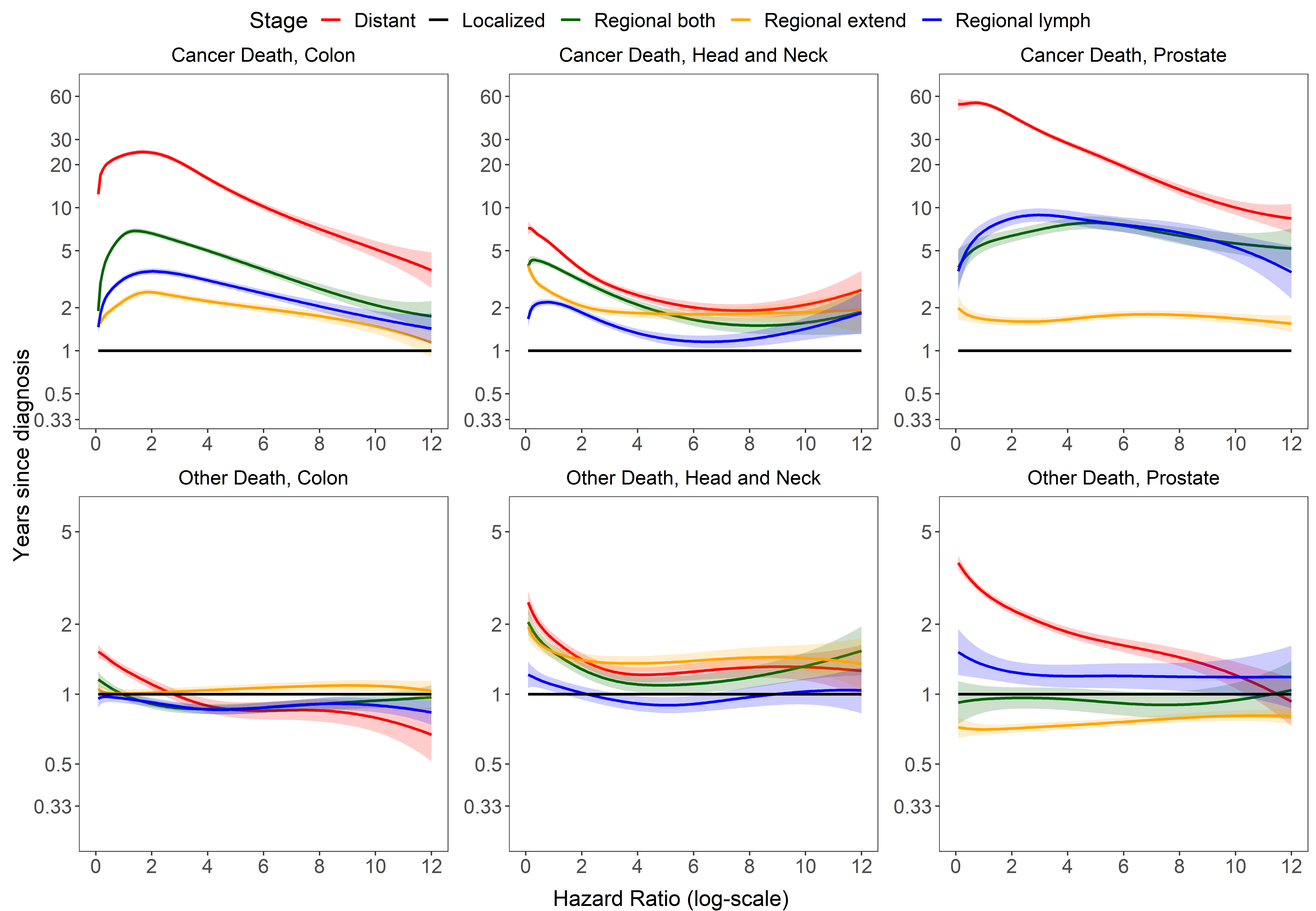

Figure 3: Time-dependent hazard ratios for stage at diagnosis, for colon, prostate, and head-and-neck cancer cancer death and other-cause death for each stage at diagnosis in multivariable models. The ribbons in all plots represent 95% confidence intervals for the estimate. Hazard ratio is shown on a log-scale.

Figure 3 shows the time-varying coefficients for each stage of colon, prostate and head and neck cancer. Results are shown for both cancer death and for death from other causes. Results are shown with $\lambda$ chosen by $\textit{TIC}$. As expected, patients with distant metastasis have a much higher hazard of death from cancer than patients with localized disease, with regional disease being in between. The proportional hazards assumption for stage is clearly not satisfied for any of these cancers, with the hazard ratios generally waning as follow-up time increases. It is also intriguing that regional stage due to tumor extension has lower hazard than regional disease due to cancer in the lymph nodes for colon and prostate cancer, but not for head and neck cancer. For non-cancer deaths the hazard ratios are much smaller, as would be expected. Again we see the hazard ratios tend to wane over time. Metastatic cancer patients with prostate cancer do appear to have a noticeably higher hazard of dying from other causes than do patients with localized disease; however, this is not the case for colon cancer. This observation, prompts further investigation into the reasons why.

​

5 Conclusion

​

REFERENCES

Ching, T., Zhu, X., and Garmire, L. X. (2018) Cox-nnet: an artificial neural network method for prognosis prediction of high-throughput omics data. PLoS computational biology, 14(4):e1006076.

Dekker, F.W., de Mutsert, R., van Dijk, P.C., Zoccali, C., and Jager, K.J. (2008) Survival analysis: time-dependent effects and time-varying risk factors. Kidney International, 74(8),994-997.

Englesbe, M., Lee, J., He, K., Fan, L., Schaubel, D., Sheetz, K., Harbaugh, C., Holcombe, S., Campbell, D., Sonnenday, C., andWang, S. (2012). Analytic morphomics, core muscle size, and surgical outcomes. Annals of Surgery, 256(2):255–261.

Genz, A., Bretz, F., Miwa, T., Mi, X., Leisch, F., Scheipl, F., Bornkamp, B., Maechler, M., Hothorn, T., and Hothorn, M. T. (2021). Package `mvtnorm’. J. Comput. Graph. Stat., 11:950-971.

Gray, R. J. (1992). Flexible methods for analyzing survival data using splines, with applications to breast cancer prognosis. Journal of the American Statistical Association, 87(420):942–951.

Hastie, T. and Tibshirani, R. (1990). Exploring the nature of covariate effects in the proportional hazards model. Biometrics, pages 1005–1016.

He, K., Yang, Y., Li, Y., Zhu, J., and Li, Y. (2017). Modeling time-varying effects with large-scale survival data: an efficient quasi-newton approach. Journal of Computational and Graphical Statistics, 26(3):635–645.

Kalantar-Zadeh, K. (2005). Causes and consequences of the reverse epidemiology of body mass index in dialysis patients. Journal of Renal Nutrition, 15(1):142–147.

Parikh, N. and Boyd, S. (2014). Proximal algorithms. Foundations and Trends® in Optimization, 1(3):127–239.

Saran, R., Robinson, B., Abbott, K. C., Agodoa, L. Y., Bhave, N., Bragg-Gresham, J., Balkrishnan, R., Dietrich, X., Eckard, A., Eggers, P. W., et al. (2018). US Renal Data System 2017 Annual Data Report: epidemiology of kidney disease in the United States. American Journal of Kidney Diseases, 71(3):A7.

Wu, W., Taylor, J. M., Brouwer, A. F., Luo, L., Kang, J., Jiang, H., and He, K. (2022). Scalable proximal methods for cause-specific hazard modeling with time-varying coefficients. Lifetime Data Analysis, pages 1–25.

Yan, J. and Huang, J. (2012). Model selection for cox models with time-varying coefficients. Biometrics, 68(2):419–428.

Zhang, H. H. and Lu, W. (2007). Adaptive lasso for cox’s proportional hazards model. Biometrika, 94(3):691–703.

Zou, H. (2006). The adaptive lasso and its oracle properties. Journal of the American Statistical Association, 101(476):1418–1429.

Zucker, D.M. and Karr, A.F. (1990) Nonparametric survival analysis with time-dependent covariate effects: a penalized partial likelihood approach. Annals of Statistics, 18(1): 329-353.